Evaluation of Preliminary Models of the Geopotential in the United States
D. A. Smith and D. G. Milbert
National Geodetic Survey, NOAA
Note: We have lost some Greek letters in the HTML translation
Introduction
As members of the Special Working Group of the International Geoid Service, we have evaluated
the preliminary geopotential models X01 through X05; computed by the joint NASA-GSFC/DMA project (Rapp and Nerem 1994). Our focus has been the behavior of these models
in the conterminous United States. In this effort, our strategy has been to compare geoid models
derived from geopotential coefficients against GPS ellipsoid heights located on optically-leveled
benchmarks. This comparison is done in two ways. In one approach, the GPS benchmarks are
compared against the geoid values obtained from what is essentially direct evaluation of the
preliminary models. This approach suffers from the omission or truncation error inherent in an
n=360 model computation. In the other approach, the point gravity and digital terrain in and
around the United States are used to compute high resolution geoid models in remove, compute,
and restore procedures about the various preliminary models. While this approach alleviates the
omission error problem, it is seen to remove portions of the geopotential model commission error.
In this report, we begin by outlining a few important points in the computation of gravimetric
quantities from geopotential coefficients. Next, we review the features of the GPS benchmark
data set that was used in evaluation of the preliminary models. We discuss the computation
procedure used to obtain the high resolution geoid models, and display results with the GPS
benchmark comparison. Then, we compare the geopotential models directly against the GPS
benchmarks, without the removal of omission error. We close the report with conclusions and
recommendations.
Geoid Height Computation
It stands to reason that if one chooses to evaluate geopotential coefficients by means of GPS on
leveled benchmarks, then one must use the utmost rigor in computation of the geoid heights from
the coefficients. Towards this goal, we have developed formulations to support the use of
geopotential coefficients computed with an arbitrary set of normal ellipsoid constants, and to
support the computation of various gravimetric quantities relative to a different, arbitrary set of
normal ellipsoid constants (which we take as GRS80). In addition, it must be recognized that the
theory used to establish the geopotential coefficients is rooted in a solution of Laplace's equation.
However, Laplace's equation only holds in a vacuum. The geoid over land is typically interior to
the Earth's topography, where Poisson's equation would operate.
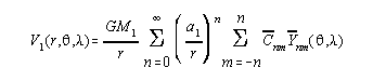
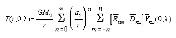
We begin by considering the evaluation of gravimetric quantities from spherical harmonic coefficients with arbitrary values of GM and a. The total external gravitational potential of the Earth can be expressed as:
where: r,,= geocentric radial distance, colatitude, longitude
GM1,a1 = scale factors associated with the Cnm values
![]() = fully normalized coefficients of the total field
= fully normalized coefficients of the total field
![]() = fully normalized Legendre functions
= fully normalized Legendre functions
And, the normal external gravitational potential of the Earth can be expressed as:
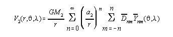
where: GM2 = Gravitation-Mass constant of the normal field
a2 = semi-major axis of the ellipsoid and which is, of itself, a "spheropotential" surface,
with constant value of normal gravity potential, Uo.
![]() = fully normalized coefficients of the normal field
= fully normalized coefficients of the normal field
(=0 if n is not positive even, or m is not zero)
The total external gravity potential of the Earth is:
W(r,,) = V1(r,,) + (r,)
and the normal external gravity potential of the Earth is:
U(r,,)=V2(r,,) +(r,)
where (r,) is the centrifugal potential.
We make the following assumptions:
1) r,, are the same in both equations, that is, the origins of the two fields coincide, as do their
three Cartesian co-ordinate axes.
2) the value of normal gravity potential on the ellipsoid (Uo), is equivalent, numerically, to the
value of total gravity potential on the geoid (Wo)
3) The total and normal centrifugal potentials are equivalent, thus the disturbing potential, will
be: T = W - U = V1 - V2
Upon evaluating the disturbing potential, we pay careful attention to the differing values of GM1 versus GM2 and a1 versus a2. We start by rewriting the equation for V1 as (and truncating the series at the given high value of 360):
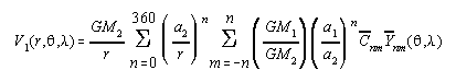
where the scaled coefficients will be expressed as:
![]() = (GM1/GM2)*(a1/a2)n Cnm = scale(n) Cnm
= (GM1/GM2)*(a1/a2)n Cnm = scale(n) Cnm
Thus:
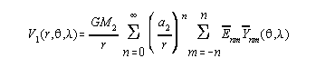
Now, with a common GM2 and a2 value "out front", we can now write the formula of the disturbing potential as:
Of primary importance here is the fact that the degree zero term is non-zero if GM1GM2. In the
case of GM1 for OSU91A (Rapp et al. 1991) versus GM2 of GRS80 (Moritz 1992), this effect is
on the order of 1 meter, in geoid undulation.
Of secondary importance is the scaling of the coefficients. The scale factors are on the order of
10-4, and this effect has been shown in some of our tests to have an RMS of 0.3 mm, with
min/max values of -0.3 mm and +0.5 mm for the geoid. While any one effect of sub-mm level will
not adversely effect our results, we feel that the number of such approximations that currently
exist in the theory need to be removed to prevent the possibility of their combined effects being
noticeable at the 1 cm level. It should be noted that this effect of properly scaling the coefficients
is not encompassed in a simple geometric transformation, but represents a fundamental correction
to the way that a spherical harmonic expansion is evaluated.
In general remarks, we are also careful about the difference between /r and /h. The
difference between the two derivatives will have small (about 5 ppm), but calculable effects, on
quantities of interest (gravity anomalies, upward derivatives of the height anomaly, etc...). And,
wherever possible, exact (closed) formulas or iterations are performed (for example, computing
the flattening from J2, , GM, and a), rather than using any approximate formulas. Considering
the speed with which iterations can be performed, we felt it was best to remove as many
approximate formulas as was reasonably possible.
Next, we consider the issue that geopotential coefficients do not accurately represent the behavior of the actual geopotential interior to the Earth's surface. This problem was raised in Rapp (1992), and amplified in Rapp (1996). Basically, one must evaluate the geopotential on or above the Earth's surface, and then develop the geoid undulation from that computation. It is convenient, therefore, to first compute height anomalies, , and then convert them to geoid undulation, N, by means of Eq. (8-10) of Heiskanen and Moritz (1967)
![]()
where
gB simple (non-terrain corrected) Bouguer anomaly .
A popular choice in geopotential coefficient evaluation is the Clenshaw summation approach
described in Tscherning, et al (1983). This implementation, however, must reform certain sums
whenever the geocentric radius, r, varies. To aid in computational efficiency, Rapp (1996)
computes the height anomaly on the ellipsoid, o, and then upward continues to the surface by the
orthometric height, H,
P = o + /r H .
In an enhancement to this approach, we perform the upward continuation by
P = o + /h h
where, after supressing a negligible dependence (0.1 ppm),
/h = (T/)/h = [(1/) T/r r/h - (T/2) /h ]
and where ellipsoidal height, h, is established by H and a preliminary geoid height, N. Note that
the second term, which contains the normal gravity gradient, /h, can be of the same magnitude
as the first term.
As additional confirmation that some type of "upward/downward" procedure is needed to
establish accurate geoid heights interior to the Earth's surface, we compare the geoid heights
computed from 2497 GPS benchmarks to the geoid heights computed from the X01 model. In
Figure 1a
, the X01 coefficients were directly evaluated at a geocentric radius, rN, which is
continually re-evaluated to conform to the geoid surface. In
Figure 1b
, our enhanced
"upward/downward" procedure is followed. Both figures incorporate the GM and a variations
discussed earlier. Comparison of the plots demonstrate clear height dependent error in Figure 1a
when one attempts to directly compute the geoid undulations interior to the Earth's surface.
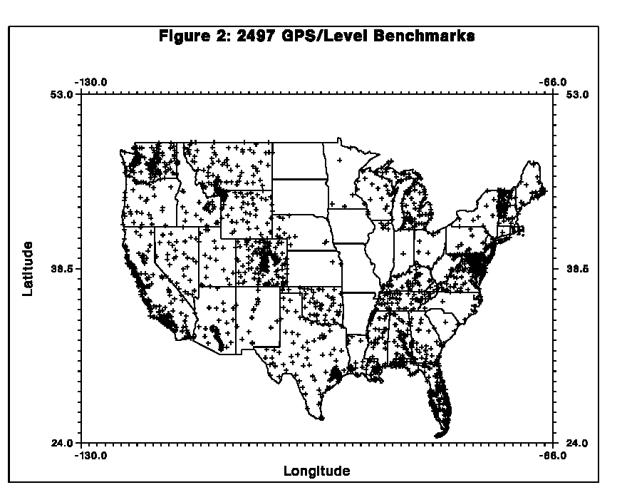
The GPS Benchmark Data Set
NGS is engaged in a project to establish a high accuracy Federal Base Network (FBN), and an
associated Cooperative Base Network (CBN), through nationwide measurement of GPS baselines
to 1 ppm accuracy or better. In the course of this survey effort, many of those FBN/CBN points
are established on NAVD 88 optically leveled benchmarks.
Figure 2
displays the locations of
2497 points that are leveled benchmarks with NAVD 88 Helmert orthometric heights, and which
have GPS measured ellipsoidal heights in the NAD 83 (86) reference system as of March 1996.
The irregular distribution illustrates the state-by-state approach to the surveying, and the different
levels of state participation.
For the purposes of the preliminary model evaluation, the NAD 83 (86) coordinates are converted
into the ITRF93(1995.0) reference frame. The transformation was performed using parameters
established by Steve Frakes, National Geodetic Survey. These parameters are summarized in
Table 1. In this paper, all ellipsoid heights are expressed relative to the GRS80 normal ellipsoid in
the ITRF93(1995.0) frame.
| Table 1 -- Transformation from NAD 83 (86) to ITRF93(1995.0) | |||
| X shift | -0.9769 | ±0.0166 | m |
| Y shift | +1.9392 | ±0.0137 | m |
| Z shift | +0.5461 | ±0.0141 | m |
| X rotation | -0.0264 | ±0.0006 | arc sec |
| Y rotation | -0.0101 | ±0.0005 | arc sec |
| Z rotation | -0.0103 | ±0.0004 | arc sec |
| scale | -0.0068 | ±0.0017 | ppm |
The NAVD 88 datum is expressed in Helmert orthometric heights, and was computed in 1991.
The network contains over 1 million kilometers (km) of leveling at precisions ranging from 0.7 to
3.0 mm/km, and incorporates corrections for rod scale, temperature, level collimation,
astronomic, refraction, and magnetic effects (Zilkoski et al. 1992). The NAVD 88 datum was
realized by a single datum point, Father Point/Rimouski, in Quebec, Canada. It must be
mentioned that there is no guarantee that the NAVD 88 datum coincides with a given normal
potential, U0. For example, Rapp (1996) found a mean offset for the NAVD 88 datum of -34 cm
relative to a U0 established by a=6378136.59. For additional details on the GPS benchmark data
set, please refer to Milbert (1995).
High Resolution Geoid Computation and Evaluation
The computation of the high resolution geoid models is based on the use of the Fast Fourier
Transform (FFT) to evaluate Stokes equation. As described in Schwarz et al. (1990), a
bandwidth-limited signal is needed for input to the FFT convolution. This mandates the use of a
remove, compute, and restore procedure; where gravity anomalies from a global geopotential
model are subtracted from gravity anomaly data, followed by convolution of the residual
anomalies into residual geoid height, and then followed by restoration of geoid heights from that
same geopotential model. Such an approach was used in the GEOID90 and GEOID93
computations for the United States (Milbert 1991, Milbert and Schultz 1993).
For the test model evaluation, a standard grid of terrain corrected, Bouguer anomalies was
generated. Now, any gridding data set is subject to aliasing in the presence of high-frequency
signal. To remove as much predictable, high-frequency content as possible, gridding is performed
on terrain corrected, Bouguer anomalies, gTB. For anomalies on land
gTB = g +![]() H -
H - ![]() H2 - + A + C - 0.1119H
H2 - + A + C - 0.1119H
where
A = 0.8658 - 9.72710-5 H + 3.48210-9 H2
and
g surface gravity, tide corrected, IGSN71 system (mgals)
H orthometric height, NAVD 88 datum (meters)
normal gravity on ellipsoid, GRS80 (Somigliana's formula) (mgals)
A atmospheric correction (Wichiencharoen 1982) (mgals)
C terrain correction from 30" elevation grid (mgals)
geodetic latitude, NAD 83 (86) datum
a semi-major axis, GRS80 (6378137 meters)
a normal gravity at equator, GRS80 (978032.67715 mgals)
f ellipsoid flattening, GRS80 (0.00335281068118)
m 0.00344978600308 (GRS80)
density of topographic masses (2.67 gm/cm3)
G gravitational constant
R mean radius of the earth
spherical distance
The gridding algorithm uses a method of continuous curvature splines in tension (Smith and
Wessel 1990) with tension parameter TB = 0.75. The method is one which honors the data and
does not display large oscillations in areas without data coverage. The standard Bouguer grid is a
3' by 3' regular grid extending from 24N to 53N and 230E to 294E (66W to 130W), and
contains 581 rows and 1281 columns. All anomalies are prefiltered by computing mean value and
mean location of the anomalies in 3' x 3' cells centered over the regular 3' latitude and longitude
intersections. This prefiltering step is recommended by Smith and Wessel to reduce spatial
aliasing effects prior to gridding.
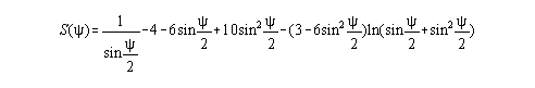
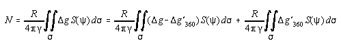
Since we are using Stokes theory to compute the geoid, we require gravity anomalies on the geoid surface, rather than at the Earth's surface. We adopt Helmert's second method of condensation to regularize the problem and include the indirect effect with Grushinsky's formula
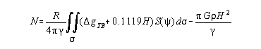
where Stokes function is
This setup is solved in a remove-compute-restore procedure using the FFT formulation of Strang van Hees (1990),
g+ = (gTB + 0.1119H)- g'360
![]()
N = N++ N'360
where
g+ high-frequency part of gravity anomalies
g'360 geopotential model gravity anomalies at geoid surface
, grid spacing
F, F-1 direct and inverse, two-dimensional, Fourier transforms
N+ high-frequency part of geoid undulations
N'360 geopotential model geoid undulations at geoid surface
and, where Stokes function, S, is evaluated with a mean latitude, m, and the approximation,
sin [sin2 (P-Q) + sin2 (P-Q) (cos2m- sin2 (P-Q)) ]
The input grid, g+, (580 rows, 1280 columns) had 50% zero padding on all four edges to
eliminate the effect of cyclic convolution (Gleason 1990). No tapering of g+ was performed,
since the long wavelength part has already been removed. The FFT subroutine has an option
which exploits the Hermitian symmetry resulting from real valued grids. Thus, doubled
computation speed and storage efficiency was obtained without resorting to Hartley transforms.
An important issue must be mentioned at this point. The geopotential model geoid undulations,
N'360, are evaluated at the geoid surface. From the results of Figures 1a and 1b, it is seen that
these geoid heights are biased. However, the Stokes procedure described above will remove that
height dependent error if the gravity anomalies, g'360, are also evaluated in a fashion consistent
with the geoid undulations. Since it is not convenient to apply some form of "upward/downward"
procedure to the gravity anomalies, we choose to evaluate both geoid and anomalies at the geoid
surface. The key point is that we are consistent in our choice of surface for coefficient evaluation.
As a formal demonstration, consider Stokes equation written in a remove, compute, and restore procedure:
The term on the right formulates the N, which must be restored, as a function of the model gravity anomalies, g'360, that were removed. Expanding Stokes function in Legendre polynomials and the gravity anomalies in terms of the harmonic coefficients yields
where ![]() . Perform the multiplication, exchange the order of the sums and
integrals, under a customary assumption of convergence, combine terms, and invoke the
orthogonality relationships of Legendre polynomimals. After algebra, the equation above will
simplify into
. Perform the multiplication, exchange the order of the sums and
integrals, under a customary assumption of convergence, combine terms, and invoke the
orthogonality relationships of Legendre polynomimals. After algebra, the equation above will
simplify into
if the leading R before the integeral is taken to be r. The equation above is equivalent to N'360.
Other than the R=r requirement of the lead term, the development did not invoke any specific
surface mandated by a remove, compute, and restore procedure. The development did show the
consistent N'360 and g'360 expressions.
The high resolution geoid models are derived from four data sources: point gravity measurements,
satellite altimetry-derived gravity anomalies, digital terrain, and geopotential coefficients. A few
remarks are appropriate. About 1.8 million gravity points, both ship and terrestrial, went into the
gridding. These data were a combination of NGS-held data and quality controlled data from the
Defense Mapping Agency. The satellite altimetry-derived gravity anomalies were computed by
Sandwell and Smith (1996). These were included in gravity void regions where depths exceeded
500 meters and which were 200 km or more from land. The digital terrain data came primarily
from the 30" point topography database, TOPO30, distributed by the National Geophysical Data
Center (Row and Kozleski 1991). The 30" elevation set was used to compute both terrain
corrections, and 3' x 3' mean elevations. And, of course, the preliminary geopotential models,
X01 through X05, were used as the coefficent sources. We denote the resultant high resolution
models as 9620 through 9624, respectively.
We explore the general properties of the solutions by computing geoid height residuals, e, in the
sense of
e = high-res. geoid height - (ITRF93(1995.0) ellipsoid height - NAVD 88 orthometric height).
Tilted plane models are fit to the 2497 residuals and are summarized in Table 2.
Model    Offset(cm.)    Tilt(ppm)    RMS about plane(cm)    Azimuth(deg)
9620       -4.58          0.04             35.07                293
9621       -5.90          0.06             36.14                317
9622       -2.07          0.05             36.14                319
9623       -2.05          0.06             36.56                321
9624       -2.05          0.05             36.52                321
Table 2. Tilted plane fits to 2497 high resolution geoid model residuals .
These results begin to indicate model differences. The average offsets suggest that X01 and X02
used differing data and/or procedures from X03, X04, and X05. The small magnitude of the
offsets must be considered in the context of the comparisons. The GRS80 normal ellipsoid is
used to express the ellipsoidal heights, the normal gravity, and the high resolution geoid models.
Thus, the small offsets are not inconsistent with the -34 cm found by Rapp (1996).
Next, following the approach of Milbert (1995), smoothed residual surfaces are computed by means of collocation for all 5 high resolution models. Empirical covariance functions were fit to the covariance statistics of the detrended geoid residuals. The fits were made using a simple function of the form
![]()
where
d = the spherical distance between points (km)
L = characteristic length (km)
C0 = function variance (m2)
The function fits were virtually identical, with only minor variations of L = 485 km and C0 =
(0.31)2 m2. As was seen in Milbert (1995), the residual error is sizable and correlated over a long
length scale. The detrended residual error, ![]() , is predicted on a 30' x 30' grid using least-squares
collocation with noise (Moritz 1980, p.102-106). The prediction formula is
, is predicted on a 30' x 30' grid using least-squares
collocation with noise (Moritz 1980, p.102-106). The prediction formula is
![]()
where
Ctt = signal covariance between observations
Cst = signal covariance between predicted signal and observations
Cnn = covariance of random measuring errors, taken as diagonal and constant: Cnn=so2 I
Before the grids are computed, the prediction process is iterated to establish a value of so2
consistent with the residual misfit about the predictions. It was found the RMS of residuals from
the prediction step matched the assigned noise when so2 = (5.6)2 cm2 for the n=2497 points. The
trends reported in Table 2 were restored to the detrended signal grids, resulting in the final
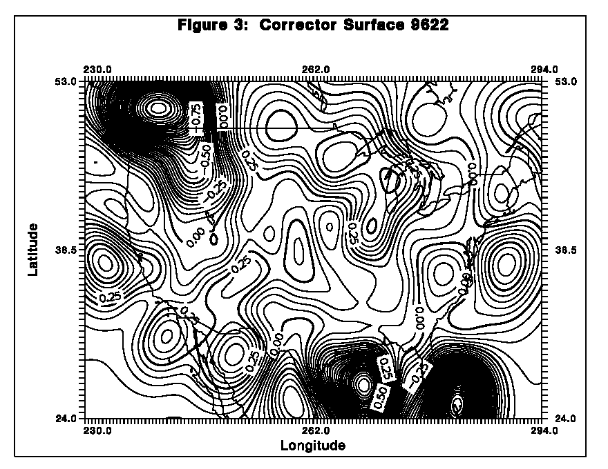
corrector surface grids (adjusted in sign to provide an additive correction).
Figure 3
portrays a trend surface that, when added to the 9622 geoid model, will directly relate
ITRF93(1995.0) ellipsoid heights and NAVD 88 Helmert orthometric heights. In viewing this
figure it must be recalled that the GPS benchmarks used to develop this grid all lie within the U.S.
borders; and that highs or lows in the oceans or in other countries are extrapolations, and are not
reliable. In the interests of concision, the trend surfaces for the other 4 models are not displayed,
since they appear almost identical.
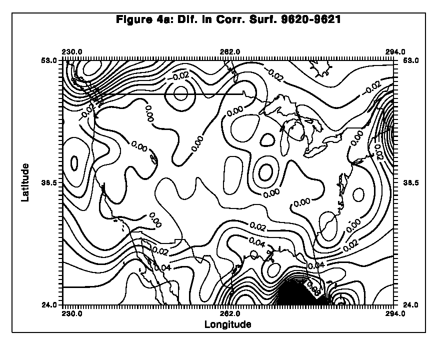
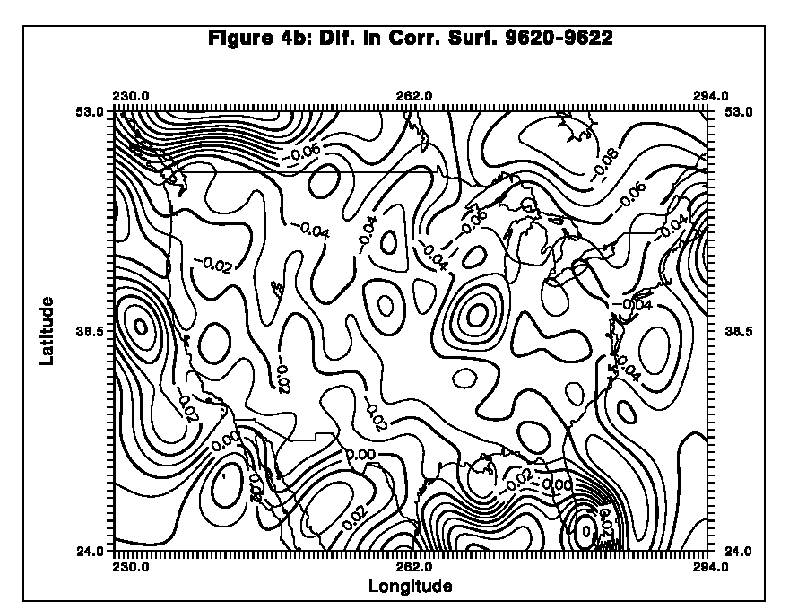
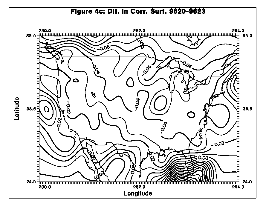
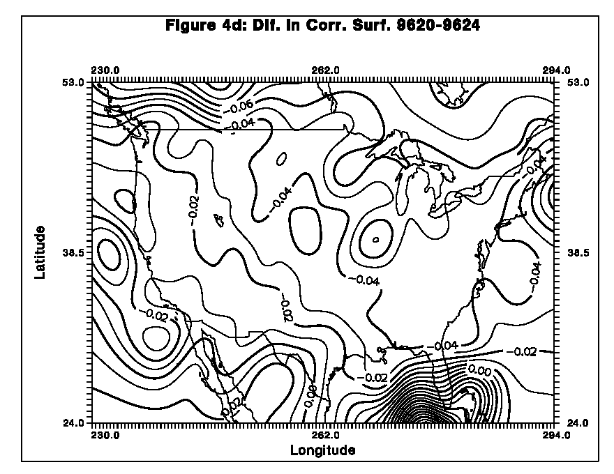
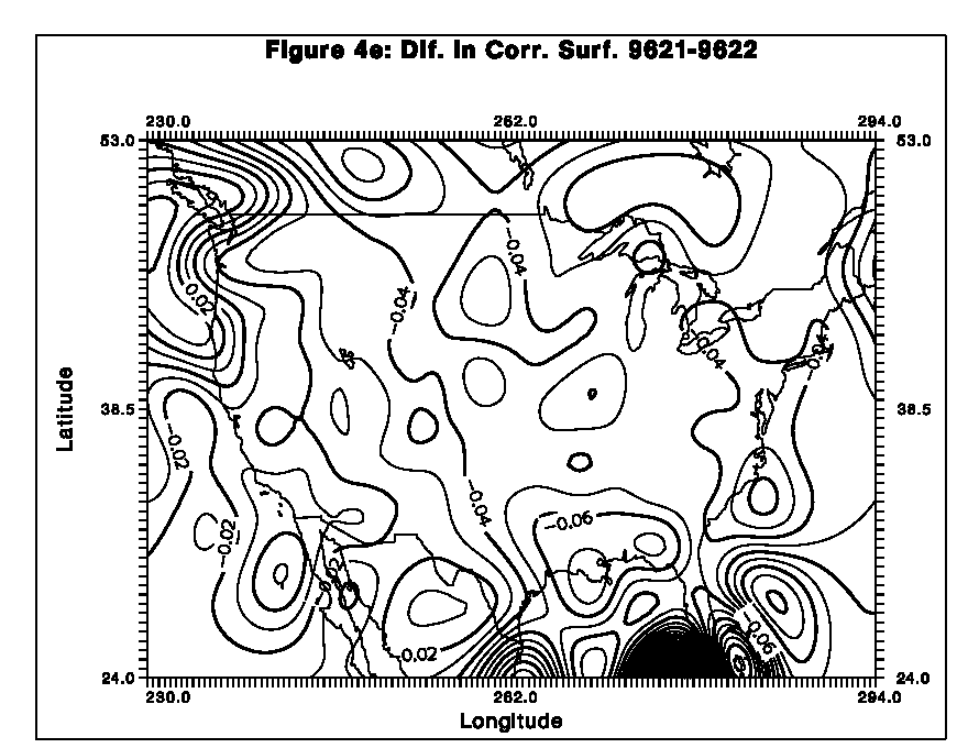
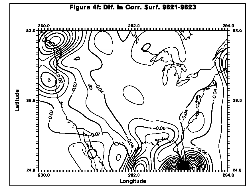
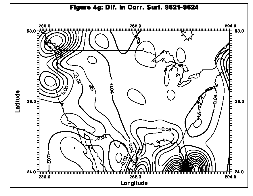
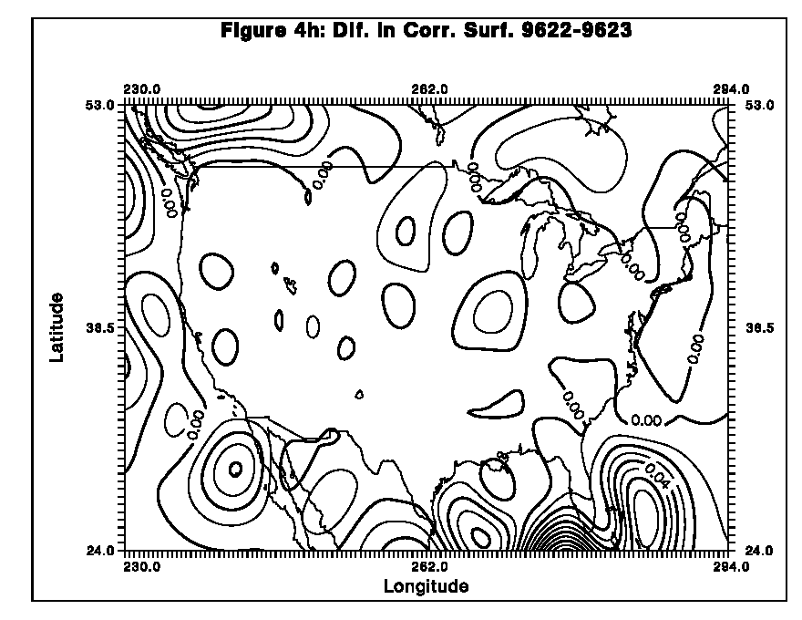
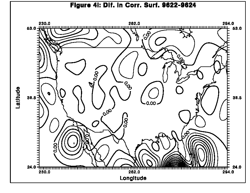
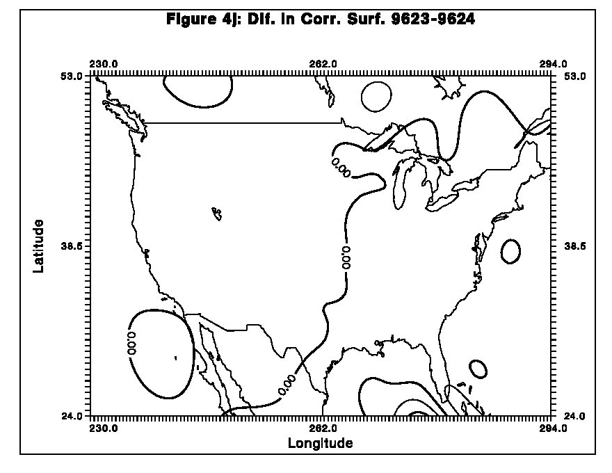
As part of the evaluation process, we computed all possible combinations of the residual trend
surface differences, 10 in all. These are reproduced in Figures 4a through 4j.
[
Figure 4a
,
Figure 4b
,
Figure 4c
,
Figure 4d
,
Figure 4e
,
Figure 4f
,
Figure 4g
,
Figure 4h
,
Figure 4i
,
Figure 4j
]
Inspection of the
combinations indicate that the 9623 and 9624 models were virtually identical, and that 9622 was
very close to the 9623 model. (One must discount features in the GPS benchmark void areas.) It
is also seen that model 9621 shows some departures from 9622, and that 9620 is the most
different of all the models. These results confirm the similarities of the 9622, 9623, and 9624
models, and also suggest that both 9620 and 9621 are distinct from them and are distinct from
one another.
At this point it is helpful to review particular features seen in the trend surfaces. A tilt is evident
in Florida, and it is virtually the same in all models. This effect has been observed with both the
GEOID90 and GEOID93 models, as well as with numerous test models. Given the great care
taken by the geopotential model computation team in the intercomparisons of marine gravity and
altimetry derived gravity, and given the very flat topography of Florida, it is unlikely that the
geoid models are the source of this feature. Further, since the GPS network is anchored to the
Richmond VLBI site at the tip of Florida, it is also unlikely that the ellipsoid heights are biased in
that region. The leveling is suspect. On the other hand, the tilt along the Gulf Coast is probably
gravimetric in origin; and will be discussed later in this section.
A North-South tilt is also evident in Washington State. The source of this feature seems to be the
terrain corrections computed from digital terrain data in southern British Columbia. We are
working with the Geodetic Survey of Canada to resolve this problem. It is thought, however, that
the mean gravity anomalies used to compute the preliminary geopotential models are accurate.
The tilt is seen to blend into an elongated feature over the northern Rockies. This raises some
concern over possible height-dependent error.
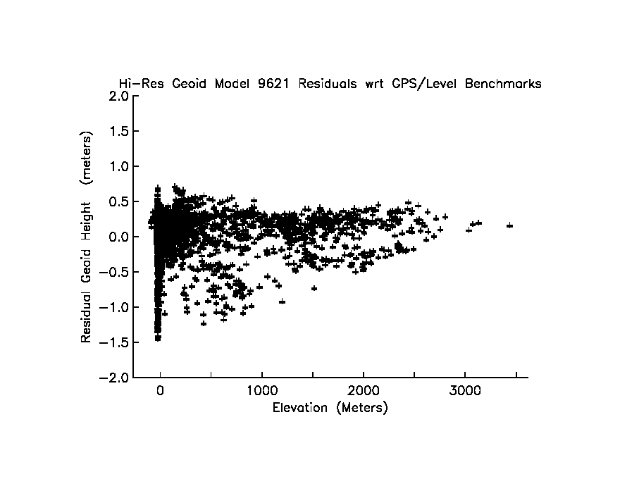
As a different view of the models, we made scatter plots of the geoid height residuals relative to
elevation. A sample for the 9621 model is given in
Figure 5
, since the scatter plots look similar.
The dispersion of values near the zero elevation reflect the issues in Florida and the Gulf Coast
noted earlier. No obvious height dependence is evident in Figure 5, unlike the effect seen in
Figure 1a
. However, overlays of the the 5 different scatter plots do show small variations that
could have an elevation dependence.
In pursuit of this possibility, an exploratory GPS benchmark data set was formed by witholding
the points in Florida south of 30N, and by witholding the points north of 48N in Washington
State. The average offset, and the RMS about the offset are then computed. In addition, the
offset and RMS are computed where data are witheld below 1000 m, below 1500 meters, and
below 2000 meters in elevation. The statistics are grouped by model, ordered by ascending
elevation, and displayed in Table 3. In addition, the differences in average offset, and second
differences are displayed.
 9620 Model      Cutoff(m)   n    RMS(cm)     Offset(cm.)   Diff   2nd-Diff
  (X01)              0     2190    24.85         9.15
                  1000      448    23.99         6.58
                  1500      268    24.98         6.32      -0.26
                  2000      107    24.79         6.70       0.38     0.64

 9621 Model      Cutoff(m)   n    RMS(cm)     Offset(cm.)   Diff   2nd-Diff
  (X02)              0     2190    24.59         9.82
                  1000      448    23.76         7.50
                  1500      268    24.71         7.15      -0.35
                  2000      107    24.51         7.57       0.42     0.77

 9622 Model      Cutoff(m)   n    RMS(cm)     Offset(cm.)   Diff   2nd-Diff
  (X03)              0     2190    24.64         9.71
                  1000      448    23.77         7.07
                  1500      268    24.78         6.92      -0.15
                  2000      107    24.50         7.46       0.54     0.69

 9623 Model      Cutoff(m)   n    RMS(cm)     Offset(cm.)   Diff   2nd-Diff
  (X04)              0     2190    24.66         9.92
                  1000      448    23.78         7.38
                  1500      268    24.77         7.26      -0.12
                  2000      107    24.47         7.83       0.57     0.69

 9624 Model      Cutoff(m)   n    RMS(cm)     Offset(cm.)   Diff   2nd-Diff
  (X05)              0     2190    24.73         9.84
                  1000      448    23.83         6.97
                  1500      268    24.80         6.88      -0.09
                  2000      107    24.50         7.43       0.55     0.64
Table 3. Geoid residual statistics ordered by elevation cutoff tolerance.
Table 3 enables us to discern more about the computation of the preliminary models. The
differences in the average offset between the 0 m elevation cutoff and the 1000 m cutoff are
probably indicative of remaining systematic errors in the GPS benchmark or in the detail gravity
data, rather than reflecting characteristics of the global models. We know that the average offset
will contain NAVD 88 vertical datum error. We don't know what that error is, but we can expect
that error to be constant with respect to elevation. Thus, we can expect a zero value for the
differences in average offset. Height dependent effects will cause variations in the average offsets
as the elevation cutoff is varied.
Looking at the offset difference column, we see that X03, X04, and X05 are distinct from X01
and X02. In fact, the close similarities suggest that X03, X04, and X05 are members of a family,
perhaps controlled by some tuning parameter(s), such as anomaly weighting. And, it seems that
the models X03, X04, and X05 are provided in sequence; corresponding to monotonic changes in
the hypothetical parameter.
At this stage it is seen that model 9624, computed from X05, displays the most uniform average
offsets.
To close this section, a result was obtained that sets the stage for the next section of the report;
where the models are directly compared against GPS benchmarks. Recall that in this section, the
geopotential models are evaluated through high-resolution geoid models computed in a remove,
compute, and restore procedure. One of the products of this procedure is the output grid from
the FFT convolution, which we denoted, N+. This grid contains the high-frequency part of the
geoid (truncation or omission error), but also contains information about lower-frequency
commission error.
One must interpret an N+ grid with caution. First, the grid, when added to the preliminary model
geoid, N360, will yield the co-geoid. One can think of the N+ grid as being biased by the indirect
effect, since Faye anomalies were used in its computation. Second, our model geoids, N360, were
biased, since they were evaluated interior to the Earth. Therefore, our N+ grids will also contain
that height-dependent bias. Despite these drawbacks, the N+ grid certainly contains useful
information at lower elevations.
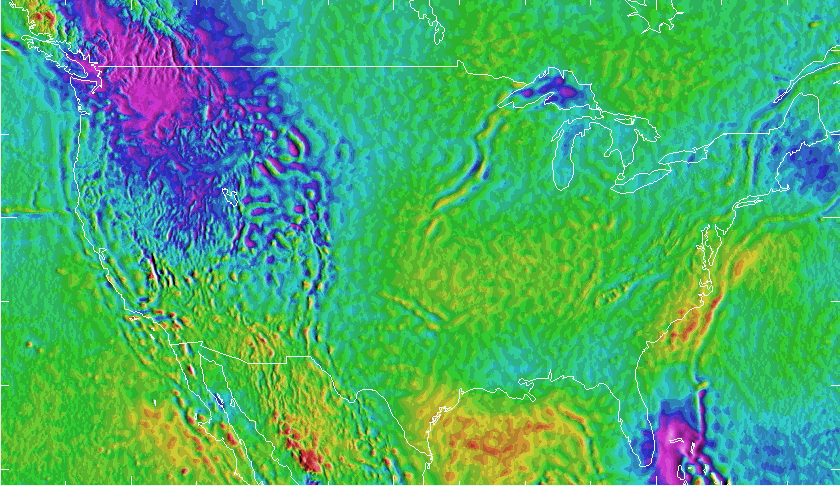
Figure 6
portrays a color shaded relief image of the N+ grid associated with the X02 model.
Sixteen hues were allocated from the low of -1.5 m (magenta) to the high of +1.5 m (red).
Sixteen levels of gray shading were added to give the effect of illumination from the East. The
magnitudes of the grid actually ranged from -4.1 m to 2.8 m. Thus, values which exceed the 1.5
meter interval will "saturate" into the magenta or the red coloring. The grids from the other
preliminary models look very similar.
Most noticable is the large blue and magenta structure in the Rockies. Because of the bias issues
discussed above, one can, at most, say that it hints at significant commission error in the Rockies.
This issue will be explored in the next section.
Other features are interesting. The lows in Lake Superior may be due to our treatment of the
elevations of the ship gravity data. The low in the Bermudas may also be related to our gravity
data set, and will be investigated at a later stage. While the Bermudas feature does induce a tilt
across Florida, it is localized to the south, and does not explain the complete amount of tilt we
have seen in the past. In addition, some portion of the low seen in Washington State and southern
British Columbia is due to currently unresolved problems with terrain corrections, discussed
earlier.
On the other hand, the 0.5 m feature in the Central U.S., and the 1 m features in the Gulf of
Mexico and off the Atlantic seaboard are less easily explained. These are regions of low
elevations, and are rather broad. The data in the Gulf and near-shore Atlantic are ship gravity
data. The altimeter-derived gravity anomalies from Sandwell and Smith (1996) were only used in
the southern part of the Gulf and in the deep Atlantic. We suspect these particular features may
be due to preliminary model commission error; perhaps correlated with some sea surface
(dynamic) topography effect in the ocean.
Low Resolution Geoid Computation and Evaluation
In this section, we compare geoid heights computed directly from the preliminary geopotential
models against the GPS benchmark data set. While these statistics are very noisy, due to
omission error, they can portray long wavelength commission error.
Five geoid grids at 3' x 3' spacing were computed from the X01 through X05 coefficients. All
grids were computed with the "up/down" procedure, where the coefficients are evaluated at the
ellipsoid, upward continued to the surface to form a height anomaly, and then converted "down"
to a geoid height by means of Eq. (8-10) of Heiskanen and Moritz (1967). This last step is
implemented as a 3' x 3' grid which has been low pass filtered to correspond to an n=360
resolution. We emphasize that these geoid grids are not subject to the height-dependent error
illustrated in
Figure 1a
.
Tilted plane models are fit to 2497 residuals about the low resolution geoid grids, and are
summarized in Table 4.
Model    Offset(cm.)    Tilt(ppm)    RMS about plane(cm)    Azimuth(deg)
 X01       -2.16          0.40             26.52                338
 X02        1.02          0.32             29.77                336
 X03        0.07          0.35             26.22                334
 X04        0.43          0.35             25.99                335
 X05        0.76          0.35             26.10                335
Table 4. Tilted plane fits to 2497 low resolution geoid model residuals .
These results are remarkable, in that they show a significant tilt to the Northwest. This confirms
the suspicion that the large blue and magenta feature seen in the Rockies in
Figure 6
is at least
partly due to preliminary geopotential model commission error. It should be be recalled that this
tilt was not evident when the GPS benchmark residuals to the high-resolution geoid models were
computed in Table 2. It appears that the high-resolution models remove not only omission error,
but also commission error.
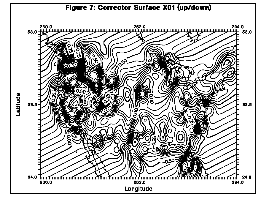
To produce an image for evaluation, smoothed residual surfaces were computed by means of
collocation for all 5 low resolution models. Empirical covariance functions were fit to the
covariance statistics of the detrended geoid residuals. The function fits were virtually identical,
with only minor variations of L = 200 km and C0 = (0.21)2 m2. The trends reported in Table 4
were restored to the detrended predicted signal grids, resulting in the final smoothed residual
surfaces. The surfaces for the 5 models were virtually identical, so only the result for model X01
is displayed in
Figure 7
.
The complex structure seen in Figure 7 is a representation of the preliminary model
omission error as sampled by the GPS benchmarks. These small features can be reduced with
more stringent smoothing, and should be ignored. Similarly, features in the oceans (e.g. near
Florida) or beyond the U.S. borders should also be ignored, since those represent extrapolations. Further, the presence or absence of structure in the central U.S. has no meaning, due to the
absence of GPS benchmarks.
However, an offset in the northern Rockies, relative to the plains, is evident in Figure 7.
Unfortunately, shortages of GPS benchmarks in the central U.S., in the Carolinas, and south of
Houston, Texas, make it difficult to comment on other features discussed in
Figure 6
. It is
noteworthy that the tilt in Florida is still evident; a result consistent with a hypothesized problem
in the level network.
To further study the behavior of the preliminary models and the possibility of commission error in
the Rockies, 505 GPS benchmarks in the region of 38- 49N and 230- 255E were extracted
from the full data set. These points were then grouped into 500 m elevation cohorts, and
statistics were computed. The statistics are grouped by model, ordered by ascending elevation,
and displayed in Table 5. In addition, the differences in average offset, and, second and third
differences are displayed. Only 15 GPS benchmarks are present in the "over 2500 m" cohort, and
those statistics are not felt to be reliable.
X01 Model   Cohort      n    RMS(cm)  Offset(cm.)   Diff  2nd-Diff  3rd-Diff
            0- 500     138    46.67     70.05
          500-1000      97    27.69     69.22
         1000-1500      93    28.78     49.63     -19.59
         1500-2000      91    31.17     35.16     -14.47     5.12
         2000-2500      71    34.38     18.02     -17.14    -2.67     -7.79
         Over 2500      15    34.92    -23.29
           ----------------------------------
              All      505    42.38     49.75

X02 Model   Cohort      n    RMS(cm)  Offset(cm.)   Diff  2nd-Diff  3rd-Diff
            0- 500     138    37.41     66.00
          500-1000      97    26.80     62.36
         1000-1500      93    29.39     49.42     -12.95
         1500-2000      91    35.50     38.88     -10.54     2.41
         2000-2500      71    30.62     23.28     -15.60    -5.06    -7.47
         Over 2500      15    37.65     -4.00
           ----------------------------------
              All      505    37.26     49.28

X03 Model   Cohort      n    RMS(cm)  Offset(cm.)   Diff  2nd-Diff  3rd-Diff
            0- 500     138    49.90     73.29
          500-1000      97    30.50     69.54
         1000-1500      93    27.14     45.97      23.57
         1500-2000      91    32.09     36.37       9.59    13.98
         2000-2500      71    32.07     19.11     -17.26    -7.67   -21.65
         Over 2500      15    36.65    -16.48
           ----------------------------------
              All      505    43.45     50.60

X04 Model   Cohort      n    RMS(cm)  Offset(cm.)   Diff  2nd-Diff  3rd-Diff
            0- 500     138    48.76     72.19
          500-1000      97    31.32     69.65
         1000-1500      93    28.26     44.36     -25.29
         1500-2000      91    32.13     35.78      -8.58    16.70
         2000-2500      71    31.75     20.01     -15.77    -7.19   -23.89
         Over 2500      15    36.04    -12.59
           ----------------------------------
              All      505    42.96     50.16

X05 Model   Cohort      n    RMS(cm)  Offset(cm.)   Diff  2nd-Diff  3rd-Diff
            0- 500     138    49.27     71.02
          500-1000      97    31.76     69.20
         1000-1500      93    28.49     42.93     -26.27
         1500-2000      91    32.98     34.90      -8.03    18.24
         2000-2500      71    29.93     18.54     -16.36    -8.33   -26.57
         Over 2500      15    35.05    -12.43
           ----------------------------------
              All      505    43.14     49.13
Table 5. Geoid residual statistics ordered by 500 m elevation cohorts.
Table 5 supports many of the conclusions developed from analysis of Table 3. Models X03
through X05 seem to be members of a family, and seem ordered relative to some tunable
parameter(s). Models X01 and X02 are distinct from that family, and from one another. Unlike
the situation in Table 3, some interpretation can be applied to the average offset column. While
we do not know the true value of the datum offset associated with NAVD 88 (in GRS80), the
high-resolution geoid model results in Table 3 indicate that it is a value closer to 10 cm than to 40
cm. This leads us to prefer models with a smaller average offset, since we feel the offset is partly
due to commission error. Models X02 and X05 look best. In general, model X05 has smaller
offsets per cohort, but shows greater height dependence of those offsets when compared to X02.
The smaller RMS about the average offsets of model X02 is also attractive.
Conclusions and Recommendations
Differencing the geoid grids computed from the preliminary geopotential model coefficients show
the test models to be very similar. So it is clear that any of the test models represents a major
advance over currently available geopotentials. With this said, we have a preference for models
X05 and X02, with a very slight edge towards X05. This preference is based on criteria of low
height dependence of geoid residuals, low average offsets of the residuals (for the case of the low-resolution models), and low RMS values. It is interesting that these criteria lead to the same
model preferences irrespective of the high-resolution or the low-resolution approach.
Since is likely that the final model will not be any one of the beta test models, it is worthwhile to
state that an ideal model would combine characteristics from X02 and X05. However, all the
preliminary models share the commission error seen in the region 38-49N, 230- 255E. If this
effect could be lessened, then the final model would be even better.
Acknowledgments
Work of this scope required the contributions of dozens of individuals. Virtually every employee
of the National Geodetic Survey has assisted in this effort. The gravity data set, the NAVD 88
project, and the GPS state upgrade program were vital to this study. The Defense Mapping
Agency (DMA) provided a major portion of the NGS land gravity data set, and was instrumental
in creation of the various 3" and 30" elevation grids in existence. Dr. Walter Smith, NOAA,
provided the altimeter-derived gravity anomalies.
References
Gleason, D.M., 1990: Obtaining Earth surface and spatial deflections of the vertical from free-air
gravity anomaly and elevation data without density assumptions. J. Geophys. Res., 95(B5), 6779-6786.
Heiskanen, W.A. and H. Moritz, 1967: Physical Geodesy. W.H. Freeman, San Francisco, 364
pp.A46-55.
Milbert, D.G., 1995: Improvement of a high resolution geoid height model in the United States
by GPS height on NAVD 88 benchmarks. In: Balmino G., F. Sano (ed), New Geoids in the
World, International Association of Geodesy, Bulletin d'Information N. 77, IGeS Bulletin N. 4,
13-36.
Milbert, D. G., and D. Schultz, 1993: GEOID (The National Geodetic Survey Geoid
Computation Program). Geodetic Services Division, National Geodetic Survey, NOAA, Silver
Spring, MD.
Milbert, D.G., 1991: GEOID90: A high-resolution geoid for the United States. EOS, 72(49),
545-554.
Moritz, H., 1992: Geodetic Reference System 1980. Bull. Geod., 66(2), 187-192.
Mortiz, H., 1980: Advanced Physical Geodesy. Herbert Wichmann Verlag, Karlsruhe, 500 pp.
Rapp, R.H., 1996: Use of potential coefficient models for geoid undulation determinations using
a spherical harmonic representation of the height anomaly/geoid undulation difference. Submitted
to Journal of Geodesy.
Rapp, R. H. and R. S. Nerem, 1994: A joint GSFC/DMA project for improving the model of the
Earth's gravitational field. Presented at Joint Symposium of the International Gravity Commission
and the International Geoid Commission, Graz, Austria, September, 1994.
Rapp, R.H., 1992: Computation and accuracy of global geoid undulation models. Proceedings of
the Sixth International Geodetic Symposium on Satellite Positioning, Columbus, Mar. 17-20,
1992. The Ohio State University, pp. 865-872.
Rapp, R.H., Y.M. Wang, and N.K. Pavlis, 1991: The Ohio State 1991 geopotential and sea
surface topography harmonic coefficient models, Report No. 410, Department of Geodetic
Science and Surveying, The Ohio State University, Columbus, OH. 94 pp.
Row III, L.W. and M.W. Kozleski, 1991: A microcomputer 30-second point topography
database for the conterminous United States, User Manual, Version 1.0, National Geophysical
Data Center, Boulder, CO, 40 pp.
Schwarz, K.P., M.G. Sideris, and R. Forsberg, 1990: The use of FFT techniques in physical
geodesy. Geophysical Journal International, 100, pp. 485-514.
Sandwell, D. T. and W. H. F. Smith, 1996: Marine Gravity Anomaly from Geosat and ERS-1
Satellite Altimetry, submitted to J. Geophys. Res.
Smith, W.H.F., and P. Wessel, 1990: Gridding with continuous curvature splines in tension.
Geophysics, 55(3), 293-305.
Strang Van Hees, G., 1990: Stokes formula using fast Fourier techniques. Manus. Geod., 15(4),
235-239.
Tscherning, C.C., R.H. Rapp, C. Goad, 1983: A comparision of methods for computing
gravimetric quantities from high degree spherical haromonic expansions. Manuscripta Geodetica,
8(3), 249-272.
Zilkoski, D.B., J.H. Richards, and G.M. Young, 1992: Results of the general adjustment of the
North American Vertical Datum of 1988. Surv. and Land Info. Sys., 52(3), 133-149.
Figure Captions
Figure 1 -- Geoid Model Residuals to GPS Benchmark Geoid Heights
a) Model X01 Evaluated at the Geoid Surface.
b) Model X01 Evaluated by an "Upward/Downward" Procedure.
Figure 2 -- 2497 Leveled Benchmarks with NAVD 88 Helmert Orthometric Heights and GPS
Ellipsoidal Heights in the ITRF93(1995.0) Reference System.
Figure 3 -- Trend Surface to Relate High-Resolution Model 9622 to GPS Benchmarks (Contour
Interval = 0.05 m).
Figure 4 -- Differences between Trend Surfaces (Contour Interval = 0.01 m)
a) through j) Differences in all Combinations .
Figure 5 -- High Resolution Model 9621 Height Residuals to GPS Benchmark Geoid Heights
Figure 6 -- High Frequency Component of Geoid Height for High-Resolution Model 9621
Relative to Preliminary Geopotential Coefficient Model X02.
Figure 7 -- Trend Surface to Relate Low-Resolution Geoid Model X01 to GPS Benchmarks
(Contour Interval = 0.05 m).
Back to the Geoid Page