The GEOID96 high resolution geoid height model for the United States
Dru A. Smith and Dennis G. Milbert
National Oceanic and Atmospheric Administration/National Geodetic Survey,
1315 East-West
Highway, Silver Spring Maryland, 20910
phone: 001- (301) 713-3202
fax: 001 - (301) 713-4172
email: dru@ngs.noaa.gov , dennis@ngs.noaa.gov
Correspondence to: D. Smith
(This paper has been published in
Journal of Geodesy, Vol. 73, No. 5, p. 219-236, 1999)
Abstract
The 2' x 2' geoid model (GEOID96) for the United States supports the conversion between NAD 83 ellipsoid heights and NAVD 88 Helmert heights. GEOID96 includes information from GPS height measurements at optically leveled benchmarks. A separate geocentric gravimetric geoid, G96SSS, was first calculated, then datum transformations and least-squares collocation were used to convert from G96SSS to GEOID96.
Fits of 2951 GPS/level (ITRF94/NAVD 88) benchmarks to G96SSS show a 15.1 cm RMS around a tilted plane (0.06 ppm, 178 degrees azimuth), with a mean value of -31.4 cm (15.6 cm RMS without plane). This mean represents a bias in NAVD 88 from global mean sea level, remaining nearly constant when computed from subsets of benchmarks. Fits of 2951 GPS/level (NAD 83/NAVD 88) benchmarks to GEOID96 show a 5.5 cm RMS (no tilts, zero average), due primarily to GPS error. The correlated error was 2.5 cm, decorrelating at 40 km, and is due to gravity, geoid and GPS errors. Differences between GEOID96 and GEOID93 range from -122 to +374 cm due primarily to the non-geocentricity of NAD 83.
Keywords: geoid, GPS, datums, reference systems, gravity
1. Introduction
Geoid models over the land can be computed by three different techniques: gravimetric, astro-geodetic, and, most recently, by differencing ellipsoidal heights and orthometric heights on leveled benchmarks occupied by GPS. The gravimetric and the GPS benchmark techniques, in particular, are highly complementary. A gravimetric geoid model can provide very high resolution and superior local accuracies, but is subject to long-wavelength (>100 km) systematic effects due to error accumulation. A network of GPS heights on leveled benchmarks has higher accuracy over long distances, but can not approach the spatial scale of gravimetric models. In theory, an optimal combination can be achieved through the integrated geodesy approach (e.g. Eeg and Krarup 1973, Milbert 1988). However, practical problems are seen when trying to apply integrated geodesy in some areas (Milbert and Dewhurst 1992).
Problems associated with data combination are highlighted in comparisons of GPS/level undulations with high resolution geoid models in the United States (Milbert 1995, Milbert 1991b). Systematic offsets, tilts, and localized discrepancies are apparent, with magnitudes ranging around +/- 1.5 meters. The source of a transcontinental tilt evident in earlier geoid models has been identified as the non-geocentricity of the NAD 83 reference frame, used to express the GPS ellipsoidal heights. However, even when one accounts for this tilt, a systematic bias between geoid undulation models and measured GPS/level undulations is seen at the 30-40 cm level. This bias is believed to be due to the offset of the NAVD 88 reference level with respect to the current best estimates of the global mean sea level (Burša 1995). With the NAD 83 tilt and the NAVD 88 bias removed, localized disagreements are still seen, at the 15.6 cm RMS level. The disagreements are probably due to errors in the geoid model, as well as older, questionable data in statewide GPS surveys.
GEOID96 represents a new era of geoid models from the National Geodetic Survey of the United States (NGS). Previous models such as GEOID90 (Milbert, 1991a) and GEOID93 (Milbert and Schultz, 1993) were gravimetric, geocentric models of the geoid. Milbert (1995) explored the possibility of computing a "biased" geoid model which would directly relate GPS heights in the NAD 83 frame to orthometric heights in the NAVD 88 vertical datum. That study led to the decision to produce both a gravimetric, geocentric geoid model (G96SSS) and a non-geocentric geoid model (GEOID96), as there were two distinct user groups, each with their own geoid needs. Pre-release results are found in (Milbert and Smith, 1996).
Section 2 discusses geoid computation from a global spherical harmonic model, EGM96 (Lemoine et al., 1997). Section 3 continues with the computation of G96SSS. In section 4 the GPS/benchmark set is described, and the use of that benchmark set in the computation of GEOID96 is found in section 5. In sections 6, 7, and 8 a comparison of GEOID96 and G96SSS to three other geoid models is made: the Canadian GSD95 model, the EGM96 model and GEOID93, respectively. The results are discussed in section 9 and the conclusions are summarized in section 10.
2. The Spherical Harmonic Model, EGM96
G96SSS was calculated using an established mathematical procedure, commonly referred to as "remove-compute-restore" (Schwarz et al., 1990). The procedure can be summarized as follows:
It can be seen that the spherical harmonic model of the Earth's geopotential plays an important role in this computational procedure. A recently released geopotential model, EGM96 (Rapp and Nerem, 1994, Lemoine et al., 1996) was chosen to be used in computing G96SSS.
EGM96 was preceded by five preliminary models (X01 - X05), and all 6 models were evaluated by the special working group (SWG) of the International Geoid Service (IGeS). Reports of the working group were made available on the World Wide Web (Sideris 1996), and are available in Bulletin #6 of the IGeS. The model evaluations (Smith and Milbert, 1997a; Smith and Milbert, 1997b) showed that EGM96 was a good model for the remove-compute-restore procedure in the United States. While local discrepancies are pointed out, it was concluded that the long-wavelength structure of the model was the most important factor in the models, and that EGM96 was shown to have the best long-wavelength structure of any of the models, when compared with 2951 GPS/leveling benchmarks in the U.S. (in the ITRF94(1996.0) and NAVD 88 reference frames).
Traditionally, geoid undulations and gravity anomalies have been computed from geopotential coefficients by evaluating a series expansion at a point on the geoid (i.e. inside the crustal masses). However, Rapp (1997) shows that computation of an undulation from geopotential coefficients is erroneous, inside the crustal masses. The traditional geopotential evaluation, used in this paper, is valid if the geoid undulations and gravity anomalies are treated consistently. Detailed discussion is presented in Appendix A.
When computing geoid undulations one must also be cautious about the treatment of the permanent tides of the Earth. The three frequently used systems, mean, zero and non-tidal (tide free) all have advantages and disadvantages. The mean tide system retains masses external to the Earth, and is therefore incompatible with the Stokes integral. For this reason, the mean tide system was not used. Although IAG Resolution No. 16 (IAG 1984) recommends the use of the zero tide system, the preponderance of data available to NGS is reduced to the non-tidal system. This includes the GPS ellipsoidal heights and NAVD 88 Helmert heights. Although arguments against the non-tidal system exist (e.g. Ekman 1996), consistency with data sources was preferred. As such, G96SSS and GEOID96 were produced in the non-tidal system.
3. The Gravimetric Geoid Model, G96SSS
The method for computing the gravimetric geoid model, G96SSS, is based on the use of the one-dimensional spherical Fast Fourier Transform (FFT) to evaluate the Stokes integral. As described in Schwarz et al. (1990), a bandwidth-limited signal is needed for input to the FFT convolution. Such bandwidth limitation is closely approximated through applying terrain corrections (removal of high frequency data) and removal of a spherical harmonic model (low frequency).
The FFT requires gridded data. Any gridding procedure is subject to aliasing in the presence of high-frequency signal. Therefore, one should remove as much predictable, high-frequency content as possible. For this reason, gridding is performed on complete (i.e. terrain corrected) Bouguer anomalies (Milbert 1995):
|
| (1) |
where
| (2) |
| (3) |
| (4) |
|
The gridding algorithm uses a method of continuous curvature splines in tension (Smith and Wessel 1990) with tension parameter TB=0.75. This value was selected to minimize the impact of gravity errors in mountains on adjacent grid points without gravity data. The method is one which honors the data and does not display large oscillations in areas without data coverage. The product is a 2' by 2' regular grid extending from 24 N to 53 N and 230 E to 294 E (66 W to 130 W). Thus, the grid contains 871 rows and 1921 columns. All anomalies are pre-filtered by computing mean value and mean location of the anomalies in 2' x 2' cells centered over the regular 2' latitude and longitude intersections. This pre-filtering step is recommended by Smith and Wessel (1990) to reduce spatial aliasing effects prior to gridding.
It is necessary to convert the grid of terrain corrected Bouguer anomalies into a grid of Helmert anomalies. As an approximation to Helmert anomalies, a grid of Faye anomalies is generated instead. Martinec, et al. (1993) state that the approximation is associated with a linear relationship between free-air anomalies and elevation. An alternative approach to obtain a Helmert anomaly can be found in Vanicek and Martinec (1994), Martinec and Vanicek (1994), Vanicek et al. (1996), and Martinec et al. (1996). However, this approach entails large computational requirements. For this reason, the Faye anomaly was used in accordance with past NGS practice (Milbert, 1991a, Milbert and Schultz, 1993, and Milbert, 1995).
In light of the preceding discussion, the geoid undulation, N, is computed through the generalized Stokes integral (Heiskanen and Moritz, 1967, pp. 102):
| (5) |
where
| (6) |
and
|
Therefore:
| (7) |
In accordance with equation (7), the authors have restored the Bouguer plate term, + 0.1119H, to the terrain corrected Bouguer anomaly grid of (1), using a grid of 2' x 2' mean elevations, yielding a grid of Faye anomalies.
Equation (7) is solved in a remove-compute-restore procedure using the "one-dimensional" FFT formulation of Haagmans et al. (1993). First, the residual gravity anomalies are computed:
| (8) |
where:
|
Then the residual co-geoid undulations are computed row-wise (i.e. for each fp) by:
| (9) |
followed by the restoration of the spherical harmonic model undulations and the inclusion of the indirect effect:
| (10) |
where:
|
and where the subscripts p and q indicate the fixed row and floating row respectively. Equation (9) must be evaluated for each row p, where 1 <= p <= n.
The input grid, Dg+, (870 rows, 1920 columns) had 50% zero padding on the east and west edges of the grid, but none on the north and south (870 rows, 3840 columns). This is because the one-dimensional (1-D) FFT procedure only performs the FFT in the east/west direction, and thus padding is only needed on those two edges to eliminate the effect of cyclic convolution (Gleason 1990). No tapering of Dg+ was performed, since the long wavelength part (Dg2,360) has already been removed. The final computation time for the 1-D FFT procedure over the conterminous United States was 18 hours, 41 minutes (wall clock).
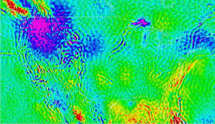
Figure 1 displays a shaded relief image of the G96SSS geoid height model. The geoid heights range from a low of -52.8 m in the Atlantic Ocean to a high of -7.7 m in the Rocky Mountains. As seen in earlier models (e.g. Milbert 1991a), significant short wavelength structure is evident.
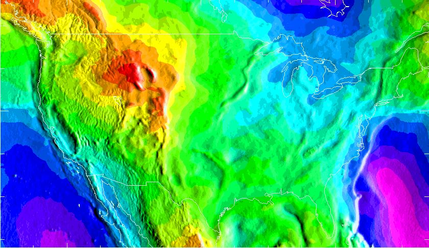
From the foregoing it is evident that the G96SSS gravimetric geoid model is derived from four data sources: point gravity, digital elevations, altimetrically derived gravity anomalies (Sandwell and Smith, 1997), and geopotential coefficients. Over 1.8 million gravity points, altimetric, ship and terrestrial, went into the gridding. The data were a combination of NGS-held data and quality controlled data from the Defense Mapping Agency (now contained in the National Imagery and Mapping Agency, NIMA). Almost all of the gravity data were on non-monumented points, and due to the consequent uncertainty in elevation, the anomalies can be considered to have a nominal accuracy of about 1 mgal. The digital elevation data came primarily from the 30" point topography database, TOPO30, distributed by the National Geophysical Data Center (Row and Kozleski 1991). The 30" point data were originally derived from 1:250,000 scale maps, and are considered accurate to 30 meters (50 meters in the mountains). In addition, an elevation grid with a 1 km nominal spacing for the Canadian Rocky Mountains was made available by the Geodetic Survey Division, Geomatics Canada on a 30" x 60" grid. This data was re-gridded to 30" x 30" and inserted into the TOPO30 Digital Elevation Model (DEM) above latitude 51 degrees north, and west of 250 degrees east longitude. The 30" elevation set was used to compute both terrain corrections (TC's), and 2' x 2' mean elevations. And, as discussed earlier, the EGM96 model was used to compute the long-wavelength gravity anomaly and geoid height grids.
As mentioned in section 2, G96SSS was computed in a non-tidal system. To establish the exact level of G96SSS, a best fitting global non-tidal ellipsoid was defined. This ellipsoid has no bearing on the final reference ellipsoid (GRS-80) used to reference the undulations, but is an altimetrically derived ellipsoid that best fits global mean sea level (within the geographic coverage of satellite altimeters). This concept is discussed thoroughly in (Rapp, 1995). At the time of our computations, an ellipsoid was used whose parameters are a=6378137.59 and 1/f = 298.25722... (yielding a W0 value of 62636855.726 m2/s2, when combined with GM=3.986004418 x 10¹⁴ m3/s2 and w = 7292115 x 10-11 rad/s). After releasing G96SSS, an improved set of best fitting ellipsoid parameters were released from NIMA. In the computation of EGM96, the NIMA/GSFC team calculated the global best fitting non-tidal ellipsoid parameters as a=6378136.46 and 1/f=298.25765, and adopted the value of W0 as 62636856.88 m2/s2. These differing values of W0 imply that the geopotential on the level surface of G96SSS differs from that of EGM96 by 1.15 m2/s2. Spatially, the separation between these two surfaces may be computed by dividing by normal gravity (which yields a constant separation of 12 cm, to centimeter accuracy). This spatial separation of the two level surfaces requires that a correction be made to G96SSS. It is necessary to subtract 12 cm from the G96SSS values to obtain the geoid undulation between the best-fit global geopotential surface (the level surface which is best fit by the EGM96 best fit ellipsoid parameters) and the GRS-80 ellipsoid (both expressed in a non-tidal system). All further references to G96SSS, especially with regard to GPS/benchmark tests, will refer to this corrected surface.
The TC's were computed on a regular 30" grid by means of the FFT convolution of Sideris (1985), but altered by the FFT formulation for spherical distance of Strang van Hees (1990), and exploiting Hermitian symmetry,
| (11) |
where
|
The grid of input heights (24- 53N, 230- 296E; 3480 rows, 7920 columns) was edge-tapered with a bell cosine function of 1 width, and then zero padded by an additional 3 width on all four edges. A 50% pad was felt wasteful, due to the rapid decay of the l0-3 kernel. Tests with a 1 km high, half Bouguer plate confirmed this rapid decay. The final TC grid was extracted from the output of equation (11), spanning the region 25- 51N, 232- 294E. Terrain corrections at all gravity points in the region were then computed with bilinear interpolation.
The use of FFT for computing TC's requires geometric approximations, and may result in some lost information at high frequencies, when compared to a rigorous prism integration. Some tests were performed in areas of rugged topography to quantify the differences between TC's computed through FFT and through prism integration. In an area of southern British Columbia, TC's at 202 gravity measurement points were investigated in the area of 50 to 51 degrees North, and 235.5 to 237.5 degrees East. Four different prism integration programs (both flat-top and slant-top types) were used as a control against the FFT terrain correction program. Using the 30" DEM, the FFT method was seen to agree with the prism methods to +/- 1 mgal at points when the prism-integrated TC was below 30 mgals. In areas where the TC's exceeded 30 mgals (some 10% of all points in the test area), the FFT program had difficulty replicating the prism integration results, and was systematically lower than them by an average of 8 mgals. It must also be understood that both FFT and prism TC's were systematically smaller than the Canadian point TC's (provided with their gravity data) in southern British Columbia. Evaluation of residual gravity anomalies and geoid undulations in the northwest U.S.A. showed significantly less signal when Canadian TC's were used, and thus Canadian point TC's were used north of 49N in computing G96SSS.
Although the FFT had trouble replicating large TC's, computer resources and time constraints meant that the 30" DEM with the FFT procedure would be used for the bulk of GEOID96. Some independent tests in southern British Columbia have shown that a systematic 8 mgal error made on TC's greater than 30 mgals has a maximum localized effect of 8 cm. While significant, it is not large enough to ascribe the predominance of geoid errors to the FFT procedure. Of greater concern is the mismatch of both FFT and prism methods with the Canadian point TC's. It is probable that high frequency information contained in the Canadian point values may not be contained in a 30" DEM. Limited prism integration tests with a 3" DEM in southern British Columbia indicate that TC's computed from a 3" DEM may nearly double the magnitude of TC's from a 30" DEM, and yet remain smaller than the Canadian provided TC's. Also, the questionable accuracy, unknown vertical datum, and sheer bulk of 3" DEM data that exists for the United States and Canada made its use too cumbersome for GEOID96. Once all preliminary TC tests were complete, G96SSS was computed using 30" TC's, and represents geoid undulations, relative to GRS-80, centered at the origin of the ITRF94 (1996.0) reference frame.
This section closes with a discussion of the computation of GEOID96 in Alaska, Hawaii, and the Puerto Rico/Virgin Island area. Gravimetric geoids were produced for these three areas using terrestrial, ship and altimetric gravity data. All three of these areas have extensive oceanic boundaries, so altimetry was of great importance to all of their calculations. To provide edge control to each grid, altimetrically derived gravity anomalies (Sandwell and Smith, 1997) were combined with ship anomalies in the ocean areas. However, detailed analysis of all ocean areas often gave precedence to the altimetry data, and (when necessary) some unreliable ship data was dropped, in preference for the altimetric data. Complex near-shore bathymetry can yield unreliable models of ocean tides, degrading the altimetrically derived gravity anomalies. Alaska, Hawaii and Puerto Rico/Virgin Islands all have complex near shore bathymetry and thus each area was thoroughly examined for how best to mix altimetry with ship data (in a way similar to that done with G96SSS). This involved weighting altimetry and ship data based on sparseness of data, near shore bathymetry, and altimetry/ship agreements. In all three areas a gravimetric, geocentric geoid was produced using the same techniques as G96SSS. However, because these three geoids were released as end-products, they were designated as GEOID96 models, rather than G96SSS. The relevant statistics for all three geoids are presented in Table 1, and are shown with the conterminous U.S. values for G96SSS, for completeness.
|
Table 1 -- Statistics for GEOID96 in Alaska, Hawaii and Puerto Rico/Virgin Islands | ||||||
|
Name |
Latitude Boundaries | Longitude Boundaries | Geoid Grid Spacing | Terrain Correction Grid Spacing | Minimum Geoid Undulation | Maximum Geoid Undulation |
Alaska |
49 - 72 N |
172 - 234 E |
2' x 4' |
30" x 60" |
-21.5 m |
21.3 m |
|
Hawaii |
18 - 24 N |
199 - 206 E |
2' x 2' |
6" x 6" |
-3.1 m |
27.7 m |
PR/VI |
15 - 21 N |
292 - 296 E |
2' x 2' |
6" x 6" |
-70.8 m |
-34.4 m |
G96SSS |
24 - 53 N |
230 - 294 E |
2' x 2' |
30"x 30" |
-52.8 m |
-7.7 m |
4. The GPS Benchmark Data Set
NGS is engaged in a project to establish a nationwide GPS network that is called the High Accuracy Reference Network (HARN). HARN station spacing and accuracy is variable; ranging from 25-100 km spacing, and around 1 ppm accuracy. Many of the HARN points are also NAVD 88 benchmarks. Clearly, these form a powerful data set for accuracy assessment and improvement of geoid models. Figure 2 displays the locations of 2951 points that are optically leveled benchmarks with NAVD 88 Helmert orthometric heights, and which have GPS measured ellipsoidal heights in the NAD 83 (86) reference system as of September 1996. The irregular distribution illustrates the state-by-state approach to the surveying, and the different levels of state participation. Further detail on the HARN's can be found in Bodnar (1990), Milbert and Milbert (1994), and Milbert (1995). It must be emphasized that the HARN ellipsoidal heights are not as accurate as one would expect from continuously operating GPS receivers.

The positioning and navigation communities require coordinates in the NAD 83 (86) datum. While being primarily a horizontal, classical network, the NAD 83 (86) was controlled by VLBI and Doppler data sets, and can be considered three-dimensional. Snay (1996, personal communication), has computed the seven parameter Helmert transformation from NAD 83 (86) to ITRF94(1996.0) with 8 points common to both reference systems. The results are summarized in Table 2. The RMS of fit was 13 millimeters (mm).
| Table 2 -- Transformation from NAD 83 (86) to ITRF94(1996.0) | |||
| Parameter | Value | Standard Deviation | Units |
| X | -0.9738 | ± 0.0261 | m |
| Y | +1.9453 | ± 0.0215 | m |
| Z | +0.5486 | ± 0.0221 | m |
| X | -0.02755 | ± 0.00087 | arc sec |
| Y | -0.01005 | ± 0.00081 | arc sec |
| Z | -0.01136 | ± 0.00066 | arc sec |
| scale | -0.00778 | ± 0.00264 | ppm |
Figure 3 portrays the datum differences between NAD 83 (86) and ITRF94 (1996.0) ellipsoidal heights referred to the GRS80 ellipsoid. It is seen that the non-geocentricity of the NAD 83 (86) reference frame induces a smooth, systematic difference in ellipsoidal heights. The values range from -0.28 to -1.64 m, and have an average tilt of about 0.3 ppm. Of particular note, this tilt is considerably smaller than the 1 to 2 ppm often seen in local intercomparisons. Summarizing, the ellipsoidal heights in the data set will contain vertical random error, and will have a long wavelength systematic error component caused by NAD 83(86) datum definition.
The NAVD 88 datum is expressed in Helmert orthometric heights (Heiskanen and Moritz, 1967, p. 167), and was computed in 1991. The network contains over 1 million kilometers of leveling at precision ranging from 0.7 to 3.0 mm/km (Zilkoski et al. 1992). For relative geoid analysis in a local region, leveling can be considered nearly error free. Accuracy assessment of leveling at a national scale is more problematic. An interesting result is that shown in Figure 8 of Zilkoski et al. (1992). Two independent leveling data sets, that of Canada and that of the United States, match at the 11 cm level or better at 14 points along the Canadian-U.S. border. While repeatability is not a measure of accuracy, this suggests that the NAVD 88 vertical datum is not tilted.
The NAVD 88 datum was realized by a single datum point, Father Point/Rimouski, in Quebec, Canada. The strategy and the value of the constraint were based on a number of factors. But, the foremost requirement was to minimize recompilation of national mapping products. Thus, there is no guarantee that the NAVD 88 datum coincides with the normal potential, U0, defined by the GRS80 system, nor with the level of global mean sea level (Burša, 1995). During the course of producing G96SSS, a comparison was made between 2951 ITRF94(1996.0) GPS measurements at NAVD 88 leveled benchmarks and G96SSS geoid heights in the conterminous United States. The results of that study indicate a mean bias for the NAVD 88 datum of -31.4 cm (±15.6 cm). The sense of the sign is that the zero level surface of the NAVD 88 datum is below the best estimate of the Earth's global geoid (mean sea) level (which also does not correspond to W=U0). This result is similar to that found by Balasubramania (1994). Also investigated was the magnitude of this bias for the Eastern and Western half of the United States, with results presented in Table 3. These results clearly indicate a nearly constant magnitude of the bias, further signifying that no tilt exists in NAVD 88.
| Table 3 -- NAVD 88 bias estimates for various areas in the United States | ||
| Area | Number of GPS/BMs used | NAVD 88 bias estimate (cm) |
| Whole U.S.A. | 2951 | -31.4 |
| East U.S.A. (lE > 260 ) | 1431 | -32.4 |
| West U.S.A. (lE < 260 ) | 1520 | -30.5 |
5. Computing the Conversion Surface and GEOID96
Based on the forgoing results, it does seem clear that both the United States national ellipsoidal height datum (NAD 83 (86)) and orthometric height datum (NAVD 88) are biased with respect to an ideal geocentric, best-fit, global reference system. In addition, the existence of 1 to 2 ppm, long wavelength, systematic errors seen in this, and earlier, geoid/GPS benchmark comparisons suggest the need of an additional model component. Collocation of geoid/GPS benchmark misclosures will model the combined long wavelength systematic errors in GPS leveling and the G96SSS model. Moreover, the combination of the error grid predicted by collocation with known datum relationships will allow development of a geoid model that will directly relate NAD 83 (86) to NAVD 88.
Modeling of the combined geoid, GPS and NAVD 88 errors begins by forming residuals, e, in the sense of
e = G96SSS geoid height - (ITRF94(1996.0) ellipsoid height - NAVD 88 orthometric height).
Next, since collocation requires centered quantities (Moritz 1980, p. 76), a tilted plane model was computed using the 2951 values of e, and this plane was removed from e to provide detrended residuals, which we denote as "l". Results are shown in Table 4.
| Table 4 -- Results from Tilted Plane Fit | |
| mean offset | -31.4 cm |
| tilt | 0.06 ppm |
| azimuth | 178 |
| RMS about the mean | 15.6 cm |
The mean offset of -31.4 cm should represent a good estimate of the bias in NAVD 88, since the GPS heights are transformed into ITRF94(1996.0) and don't, therefore, contain the non-geocentric bias of NAD 83(86). In addition, the lack of an east/west tilt indicates that there is no strong longitudinal, and, therefore, no strong height, dependence in the NAVD 88 datum bias (due to the strong east/west component of heights in the United States).
Figure 4 displays an empirical covariance function fit to the covariance statistics of the detrended geoid residuals. The fit is made using a simple function of the form
| (12) |
where

|
In Figure 4, the solid line indicates a function fit of L = 400 km and C0 = (0.095)2 m2. The plus symbols display the covariance statistics. It is seen that the residual error is sizable and correlated over a long length scale. Thus, this error (or errors) is a smooth, slowly-varying effect; but of a magnitude which exceeds our expectations of possible systematic effects in leveling and GPS. The dominant sources of this error are likely in the gravity data, in the digital elevations, and in the approximations to the true Helmert anomaly. Commission error in EGM96 is not a major contributor to the signal in Figure 4, because commission error over spatial scales of the grid size and smaller are removed by using surface gravity. See Smith and Milbert (1997b).
The detrended residual error, ![]() , is predicted on a 30' x 30' grid using least-squares
collocation with noise (Moritz 1980, p.102-106). The prediction formula is
, is predicted on a 30' x 30' grid using least-squares
collocation with noise (Moritz 1980, p.102-106). The prediction formula is
| (13) |
where
|
Before the grid is computed, the prediction process is iterated to establish a value of so2 consistent with the residual misfit about the predictions of equation (13). It was found the RMS of residuals from the prediction step matched the assigned noise when so2 = (5.5)2 cm2 was used for the n=2951 points. This signal grid is seen in Figure 5 and represents centered, detrended residuals between ITRF94(1996.0) GPS ellipsoid heights, NAVD 88 Helmert orthometric heights and G96SSS geoid heights. In viewing Figure 5, it must be recalled that the GPS benchmarks used to develop this grid all lie within the U.S. borders and that highs or lows in the oceans or in other countries are extrapolations, and are not reliable. To compute the total conversion surface between G96SSS and GEOID96, the trend reported in Table 4 is restored to the detrended signal grid, which is then added to the ITRF94(1996.0) to NAD 83(86) grid (Figure 3). This results in the final conversion grid (adjusted in sign to provide a subtractive conversion). Included in this conversion grid is the 12.0 cm correction that refers G96SSS to the global best-fit non-tidal system, as well as the 31.4 cm NAVD 88 datum offset. This combined grid is shown in Figure 6.
Figure 6 portrays a conversion surface that, when subtracted from the G96SSS geoid model, produces the final geoid model, GEOID96. The GEOID96 model will directly relate NAD 83 (86) ellipsoid heights and NAVD 88 Helmert orthometric heights. Figure 6, like Figure 5 is not reliable outside the boundaries of the conterminous U.S. With this in mind, it is seen that the predominant effect is a tilt in the northwest-southeast direction (being mostly the transformation between ITRF94(1996.0) and NAD 83 (86)). The conversion is smooth within the U.S. (gradients under 4 ppm) and seldom exceeds a meter.
To test the computational process leading to GEOID96, residuals were computed between the GEOID96 model and the measured geoid heights at the 2951 GPS benchmarks (this time, in NAD 83(86)). The RMS was 5.5 cm, with no offset or trends applied. Thus, the conversion process is seen to be successful.
Of particular interest, the covariance statistics for the GEOID96 model residuals were computed, and an empirical covariance function of the form of equation (12) was then developed. These results are portrayed in Figure 7. Unlike Figure 4, which was plotted to a distance of 1000 km, Figure 7 is only plotted to a distance of 100 km. At this closer scale, a drop is seen in the statistics from C = (0.055)2 m 2 at d = 0, down to C = (0.025)2 m 2 at d = 5 km. This reduction is evidence of an uncorrelated (white-noise) process. For this reason, the empirical covariance function is fit to the remaining, correlated signal; yielding L = 40 km and C0 = (0.025)2 m2.
A major source of the 5.5 cm of uncorrelated error is undoubtedly error in the GPS ellipsoidal heights. Both geoid height and leveling errors are correlated, and leveling is much too precise to contribute significantly to the value. Free-air gravity anomalies are well known in the U.S. (1 to 2 milligal), and Parks and Milbert (1995) report a relationship of 3 to 4 mm of geoid error to a milligal of gravity error when using 3' x 3' high resolution geoid models. In addition, the 5 cm uncorrelated error process is seen in both low and high elevation areas of the United States. As mentioned earlier, error in the GPS ellipsoid heights of the data set was expected. The 5.5 cm magnitude is consistent with those field survey and reduction procedures.
The correlated error is difficult to interpret. It could be correlated GPS error, lower order leveling error and geoid error from gravity data error and approximations. For example, standard errors of Second-Order leveling can range from 2.1 to 3.0 mm/km, or about 1.5 to 2.1 cm over 50 km (Zilkoski et al, 1992). It is notable that the GPS HARN network spacing is about 50 km. This may be related to the correlation length.
6. Comparison to Canadian geoid model, GSD95
While the goal of GEOID96 is to provide a high-resolution geoid model for the United States, the computational area extends about 400 km north into Canada to reduce the possibility of edge effects. This overlap provides a comparison area between U.S. geoid models and Canadian geoid models. The most recent Canadian geoid, GSD95 , was produced at the Geodetic Survey Division, Geomatics Canada (GSD/GC) in 1995 (Véronneau, 1997). It is a model of geoid undulations in 5' x 5' grid cells, extending south into the United States to latitude 42 degrees North, and was computed with slightly different procedures than GEOID96. To compare GEOID96 to GSD95, GEOID96 was interpolated onto the same grid as GSD95, and the overlapping areas of 42N to 53N, 230E to 294E were compared.
The first comparison is between G96SSS and GSD95, as they are both purely geocentric, gravimetric geoid models, with no GPS/benchmark information used in their computation. Figure 8 shows a plot of the differences G96SSS minus GSD95, with magnitudes ranging from -2.16 meters to +0.21 meters (no bias removed). However, the north and south edges of this grid may be influenced by edge effects from the computation of G96SSS or GSD95. A general tilt exists in these differences of approximately 0.28 ppm at an azimuth of 67 degrees. This translates into a roughly 1.25 meter tilt in the east/west direction, over the span of 230 to 294 degrees longitude. Even if one removes this trend, the large features (about 1 meter in magnitude) covering Washington, Oregon, Idaho and western Montana remain. This large disagreement may be due to NGS and GSD/GC using different terrain correction sources between latitudes 42N and 49N.
If one were to examine the differences between GEOID96 and GSD95, one would be influenced by the NAD 83/ITRF94 tilt, and the NAVD 88 bias. If, however, one were to remove these two known biases from GEOID96, that would leave a geoid model that is a combination of G96SSS and GPS/benchmarks in a geocentric reference frame. This model is denoted (for the purposes of this comparison) as "G96BM". Figure 9 shows the differences G96BM minus GSD95. If one compares Figure 9 to Figure 8 it can be seen that the influence of GPS/benchmarks has changed the differences in a few areas. Specifically, notice that in Figure 8, the agreement from central Montana (48N, 255E) to western Wisconsin (45N, 270E) is good, but the addition of GPS/benchmark data yields a worse agreement as seen in Figure 9. Leveling errors of this magnitude are not likely, however it is possible that there are errors in the GPS measurements in eastern Montana In addition, the magnitude of tilt between the two models has not changed. This indicates that G96SSS is not tilted relative to the GPS/benchmarks. It may therefore be inferred that a tilt does exist between the GPS/benchmarks and GSD95.
In addition, if one looks at eastern Washington and Idaho, it can be seen that the GPS/benchmark data removes some of the disagreement between G96SSS and GSD95, making it appear to be an improvement. However, the source of the disagreement in Figure 8 is not entirely clear, and the lack of confidence in the GPS data to the east and west of Idaho makes it difficult to trust the GPS data in Idaho itself. Therefore, it cannot be stated with confidence that the GPS data in Idaho are improving or degrading the gravimetric geoid.
7. Comparison with EGM96
Geoid undulations have often been computed from geopotential coefficients (e.g. Rapp, Wang and Pavlis, 1991; Rapp and Pavlis, 1990). Lately, however, potential coefficients, augmented by 30'x30' gridded Bouguer anomalies, have been used to compute more accurate geoid undulation estimates (Rapp, 1997; Rapp, 1992). Using this procedure, undulations were computed on a 15' x 15' grid by the EGM96 team, and made available on the World Wide Web. Using this base grid, the EGM96/Bouguer geoid grid was interpolated down to 2'x2', to have a consistent grid size. Although the grid is 2' x 2', the information content of EGM96 is such that features smaller than 30' x 30' will not be contained in the grid. However, if one compares features larger than 30' x 30' between the EGM96 grid and G96SSS, areas where the surface gravity data (which yields G96SSS) differs from the gravity information contained in the potential coefficients (which yield the EGM96 grid) will be obvious.
Figure 10 shows a plot of the differences G96SSS minus EGM96, with values ranging from -185 cm in magenta to 334 cm in red. These values average -0.3 cm, with a standard deviation of 39 cm. A number of large signals are immediately obvious in Figure 10, but the largest in area is clearly the Pacific Northwest. In this area, undulation differences reach -185 cm. This disagreement may be due to the use of different DEM data, different methods of computing TC's, different sources of gravity data, or different gravity reduction techniques. As an independent check, the two geoid models (EGM96 and G96SSS) were separately compared to GPS/benchmark data in the Pacific Northwest (40 - 49 N, 235 - 245 E - the area of largest disagreements between the two models). The statistics of the comparisons show, relative to 215 GPS/Benchmarks, a G96SSS average offset of 21 cm, with a standard deviation of 22 cm. For EGM96, those numbers change to 119 cm, with a standard deviation of 37 cm. The higher standard deviation in the EGM96 comparison can be attributed to the lack of high frequency data (omission error) in the EGM96 grid. However, the clear 98 cm difference in the average offset indicates that, there is a nearly one meter bias in the EGM96 geoid undulations in this area.
In the Gulf of Mexico, differences between G96SSS and EGM96 are pronounced, with magnitudes as large as 135 cm. Altimetry derived gravity anomalies (Sandwell and Smith, 1997) were used in the western half of the Gulf of Mexico, and ship data in the eastern half. The computation of EGM96 also used altimetry, but for anomalies as well as direct undulation measurement, with the solution of an ocean dynamic topography model as well. The ocean dynamic topography (difference between the sea surface and geoid) is at the 40-120 cm level in the Gulf of Mexico (Wang and Rapp, 1993). Although Sandwell and Smith (1997) use high pass filtering to remove some dynamic topography effects, the actual dynamic topography is not directly removed from the altimeter signal in the spatial domain, and what is seen in Figure 10 may be its effect. However, this does not explain the large differences in the east half of the Gulf, where ship data were used.
Further comparisons between EGM96 and G96SSS were performed at NGS for the SWG of EGM96, but these are not outlined here. Full details may be found in (Smith and Milbert, 1997b).
8. Comparison with GEOID93
GEOID93 (Milbert and Schultz, 1993), like its predecessor GEOID90 (Milbert, 1991a), is a gravimetric, geocentric geoid model, and a comparison between GEOID93 and G96SSS will show where our new data, and new geoid computational methods have changed the estimate of the geoid undulation. However, GEOID93 served as the geoid model for converting GPS heights to orthometric heights, and should also be compared to GEOID96 to show the significance of the conversion surface. Figure 11 shows the differences GEOID96 minus GEOID93. These differences range in magnitude from -1.22 meters up to 3.74 meters. The dominant feature of these differences is the northwest tilt due to the transformation between NAD 83 and ITRF94. The -31.4 cm bias in NAVD 88 is another difference between GEOID93 and GEOID96. Significant changes in the terrain data in southern British Columbia, as well as gravity data in the Bahamas and the western Gulf of Mexico are all responsible for the large changes seen in those areas. Finally, high-frequency differences in the entire ocean domain can be seen, which is due to the inclusion of altimetrically derived gravity anomalies in computing GEOID96.
Note the significant tilts induced across Washington State and Florida, due to corrections made in southern British Columbia and the Bahamas respectively. These tilts were seen when GEOID93 was compared to GPS on NAVD 88 benchmarks, and have now been significantly reduced in GEOID96, but as seen in Figure 6, these features are still far from eliminated.
9. Discussion
Figures 4 and 7 show the covariances of the differences between the GPS benchmarks and the G96SSS and GEOID96 model, respectively. The remarkable change between these two figures demonstrates the effectiveness of the collocation procedure. The detrended, correlated error was reduced from an RMS of 15.6 cm (Table 4), to an RMS of 2.5 cm, in the presence of 5.5 cm RMS Gaussian noise (Figure 7). Further, this result was obtained from a very smooth empirical covariance function of L=400 km. The error present in the GPS benchmark residuals, e, (which have geoid model, NAVD 88, and GPS sources) fell into two distinct spectral domains: long-wavelength (~400 km) and short-wavelength (~40 km).
The long-wavelength error sources can be partially identified by inspection of the prediction grid. Since the conversion surface of Figure 6 is dominated by the datum difference between ITRF94(1996.0) and NAD 83(86), interpretation of the detrended, centered residuals of (Figure 5) is performed.
Figure 5 is only valid over land,with few GPS benchmarks contributing to its character in the central U.S. The dominant structure is an east-west tilt in the Pacific Northwest area (centered around 45N, 245E), which then slopes back down across western Montana. While the western part of Washington State is mountainous, the eastern part contains the Columbia Basin (47N, 241E) and is fairly flat, yet it shows greater tilt. In addition, other states which have equivalent or greater relief and which are well-sampled by GPS benchmarks, such as Colorado, show less structure. This discrepancy may be related to G96SSS model problems in southern British Columbia. However, with the addition of new digital elevation data, and the use of Canadian TC's in southern British Columbia, the source of geoid error in this area is elusive. The signal is much too large to be solely due to NAVD 88 leveling error.
The high in Figure 5 centered over the northeast corner of Montana is likely due to GPS ellipsoid height error. The G96SSS model agrees well with the GSD95 model (Figure 8) in the region. However, when the GPS benchmark data are included, then the high is generated (Figure 9). Because of the very benign topography in the area, it is not realistic to assume that the agreement before the addition of GPS data was due to a common geoid error in both G96SSS and GSD95. More likely, G96SSS is reasonable in this area, and the collocation procedure has transferred long wavelength systematic error from the GPS heights into the conversion surface and the GEOID96 model in that region.
On the other hand, note the tilt seen in the southern half of Florida in Figure 5. This represents a reduction of the tilt seen throughout the entire state in Figure 7 of Milbert (1995). During computation of the G96SSS model, it was found that the older, statewide tilt was caused by a lack of gravity coverage in the Bahamas region. The addition of satellite altimetry close to land in that region improved the geoid model in Florida. Recently, the remaining southern Florida tilt of Figure 5 has been traced to ship gravity, incorrectly coded as land gravity data south of Florida. Therefore, this tilt in Florida exemplifies an improvement to the G96SSS model by the GPS benchmark data.
Next, consider the Gulf of Mexico. The sign of the tilt along southern Louisiana and the Gulf coast of Texas is consistent with subsidence. While some areas along the Gulf coast are known to subside at over 1 cm /year, the overall magnitude in Figure 5 is too large to be solely due to subsidence. The magnitude of the tilt along the west half of the Gulf of Mexico has been reduced from that seen in GEOID93 and Milbert (1995). This reduction was accomplished by the inclusion of altimetric gravity anomalies in the near shore areas of the Gulf of Mexico, west of New Orleans. However, because of the introduction of altimetric anomalies, G96SSS disagrees with EGM96 in the Gulf of Mexico. However, the agreement with GPS/benchmarks was our primary goal. Again, the tilts in the Gulf coast region (Figure 5) exemplify improvement to the G96SSS model by the GPS benchmark data.
A broad, 10-40 cm feature is seen in Figure 5 near the Great Lakes, over Minnesota and Wisconsin. However, there are relatively few GPS benchmarks in this area. The GPS survey in Wisconsin dates from 1991, and was designed for horizontal accuracy requirements. While the mid-continent gravity high is in the region, it is a narrow, linear feature, and is perpendicular to the elongation of the broad feature. The density variation of the Great Lakes was not incorporated in the computations, but Martinec et al. (1995) show the effect to be in the vicinity of 1 cm. Nonetheless, it is suspected a portion of this feature is related to gravity data/reduction in Lake Superior.
In general, it can be seen that the majority of signal of Figure 5 is commission error in G96SSS. It is highly likely that most of this commission error is due to data errors, as opposed to shortcomings in theory. One expects the greatest impact of approximations to be in the mountains. But, many features in Figure 5 are found in areas of very low topographic relief. Certainly, a major feature is found in the mountainous northwest United States. But, the topography south of 40 N has equivalent roughness, even higher elevations (e.g. the Colorado Rockies), and does not show major features in Figure 5. If use of a Faye anomaly causes large problems, then it should fail throughout the Western U.S., and not just in the northwest corner. This is not to say that the substitution of a Faye anomaly for a rigorous Helmert anomaly is ideal (Martinec, et al., 1993, eq. 34). Rather, the data errors are masking the effect of using Faye anomalies. At this time, no study exists which compares Faye anomalies to more elaborate Helmert anomalies at the geoid, or which compares GPS on benchmarks to a geoid computed from Helmert anomalies. The magnitude of a Faye anomaly approximation on the geoid is an open problem. It is expected that when the data errors are resolved one will see less commission error, and that the commission error will be more closely correlated to topographic relief.
In closing this section, a few remarks can be made on the computation technique for GEOID96. In one sense, the procedure may be viewed as a variant form of the integrated geodesy approach, where an empirical covariance function now substitutes for the computationally inaccessible cross-covariance matrix of the gravity data and the associated geoid. On the other hand, the empirical covariance function is quantifying systematic error, rather than random error. The peak of the empirical covariance function is 9.5 cm (Figure 4), whereas random error propagation of 1 mgal gravity data would probably result in 1 to 2 cm or better geoid height precision (Kearsley 1986, Parks and Milbert 1995). The collocation procedure used to compute GEOID96 was constructed to accommodate datum discrepancies and long wavelength systematic errors. Large scale systematic error in GPS height can be transferred into the GEOID96 model by this procedure. This is actually a desirable property, since users will establish subsequent coordinates using that same erroneous control. The systematic effects in GEOID96 will compensate, leading to accurate orthometric heights. This does imply that large scale readjustments of the ellipsoidal height network will have to be accompanied by corresponding upgrades to GEOID96-type models.
10. Conclusions
A gravimetric, geocentric geoid model, G96SSS, was computed by means of a 1-D FFT convolution about the EGM96 spherical harmonic model of the geopotential. Comparison with 2951 ITRF94(1996.0) GPS benchmarks with NAVD 88 Helmert orthometric heights identified a 15.6 cm RMS variation about a tilted plane with a mean of -31.4 cm and a North/South trend of 0.06 ppm. If one considers ITRF94(1996.0) as geocentric, this indicates a vertical datum bias of -31.4 cm in NAVD 88. No east/west trend is evident in the NAVD 88 offset. In addition, essentially the same NAVD 88 offset is obtained by fits to regionally clustered subsets of GPS/level benchmarks. A simple, empirical covariance function with a long characteristic length, L=400 km, was found to fit the detrended differences between the geoid model and the GPS benchmarks.
The least-squares collocation predictor led to the development of a smooth signal surface. Adding this surface to the -31.4 cm offset and 0.06 ppm trend, as well as the known ITRF94(1996.0) to NAD 83 (86) surface yielded the final conversion surface. Removing this surface from the G96SSS geoid model produced a new geoid model, GEOID96. This model is relative to a non-geocentric ellipsoid, and relates the NAD 83 (86) datum to the NAVD 88 datum. The differences between GEOID96 and NAD 83 (86)/NAVD 88 GPS benchmarks have a 5.5 cm RMS. Analysis of the covariances indicates the 5.5 cm value is Gaussian noise, and is likely due to random error in the GPS ellipsoidal heights. The figure is more than double the error ascribed to geoid and/or leveling, and highlights the need to improve GPS ellipsoidal height accuracies. Evaluation of the covariances of the differences between GEOID96 and the GPS benchmarks indicates a geoid accuracy of 2.5 cm with an empirical covariance function characteristic length of L=40 km.
Because of the smooth character of the collocation surface and the datum transformations comprising the conversion surface, the GEOID96 model retains the high relative accuracy of G96SSS, in wavelengths shorter than 400 km. The collocation procedure was seen to remove systematic errors in the G96SSS model, such as poorly covered regions across the country and improperly coded gravity data in the Florida region. However, the technique was also seen to add error in locations with isolated, unreliable GPS heights, specifically in the area of Montana and North Dakota.
Acknowledgments
This study incorporates the contributions of numerous NGS employees involved in the creation and evaluation of the gravity, NAVD 88, and GPS data sets. The National Imagery and Mapping Agency (NIMA, formerly DMA) provided a major portion of the NGS land gravity data, and was instrumental in the creation of various 3" and 30" digital elevation data grids in use today. NIMA was also a partner in a joint project with Goddard Space Flight Center, that developed the EGM96 global geopotential model. The Geodetic Survey Division of Geomatics Canada supplied the GSD95 geoid height model, as well as gravity and digital terrain data for comparisons. Dr. Walter Smith, NOAA, provided altimeter-derived gravity anomalies used in the G96SSS and GEOID96 models. The authors wish to thank the reviewers for their constructive comments.
References
Balasubramania, N., 1994: Definition and realization of a global vertical datum. Report No. 427, Department of Geodetic Science and Surveying, The Ohio State University, Columbus, OH. 112 pp.
Bodnar, A.N., 1990: National geodetic reference system statewide upgrade policy. Technical Papers of ACSM-ASPRS Fall Convention, Nov. 5-10, 1990, pp. A71-82
Burša, M, 1995: report of Special Commission SC3, Fundamental constants, International Association of Geodesy, Paris.
Eeg, J. and T. Krarup, 1973: Integerated Geodesy. The Danish Geodetic Institute, Internal Report No. 7, Copenhagen.
Ekman, M., 1996: The permanent problem of the permanent tide: What to do with it in geodetic reference systems? Marees Terrestres, v. 125, pp. 9508-9513.
Gleason, D.M., 1990: Obtaining Earth surface and spatial deflections of the vertical from free-air gravity anomaly and elevation data without density assumptions. J. Geophys. Res., 95(B5), 6779-6786.
Haagmans, R., E. de Min, and M. van Gelderen, 1993: Fast evaluation of convolution integrals on the sphere using 1-D FFT, and a comparison with existing methods for Stokes' integral. Manus. Geod., 18(5), 227-241.
Heiskanen, W.A. and H. Moritz, 1967: Physical Geodesy. W.H. Freeman, San Francisco.
IAG, 1984: The Geodesist's Handbook 1984. Bulletin Geodesique, 58(3).
IGeS, 1997: International Geoid Service, Bulletin no. 6, The Earth Gravity Model EGM96: Testing Procedures at IGeS, Politecnico di Milano, Italy.
Kearsley, A.H.W., 1986: Data requirements for determining precise relative geoid heights from gravimetry. Journal of Geophysical Research, 91(B9), 9193-9201.
Lemoine, F.G. et al., 1997: The development of the NASA GSFC and NIMA joint geopotential
model. Gravity, Geoid and Marine Geodesy, International Symposium No. 117, Tokyo, Japan,
September 30- October 5, 1996 (GraGeoMar 1996), Springer Verlag, 1997.
http://cddis.gsfc.nasa.gov/926/egm96/egm96.html
http://www.nima.mil/geospatial/products/GandG/wgs-84/geos.html
Martinec, Z., C. Matyska, E. W. Grafarend, and P. Vanicek, 1993: On Helmert's 2nd condensation method. Manus. Geod., 16(5), 417-421.
Martinec, Z. and P. Vanicek, 1994: Direct topographical effect of Helmert's condensation for a spherical approximation of the geoid. Manus. Geod., 19(5), 257-268.
Martinec, Z., P. Vanicek, A. Mainville, and M. Véronneau, 1995: The effect of lake water on geoidal height. Manus. Geod., 20(3), 193-203.
Martinec, Z., P. Vanicek, A. Mainville, and M. Véronneau, 1996: Evaluation of topographical effects in precise geoid computation from densely sampled heights . J. Geodesy, 70(11), 746-754.
Milbert, D.G., 1988: Treatment of geodetic leveling in the integrated geodesy approach. Report 396, Department of Geodetic Science and Surveying, The Ohio State University, Columbus, OH, 138 pp.
Milbert, D.G., 1991a: GEOID90: A high-resolution geoid for the United States. EOS, 72(49), 545-554.
Milbert, D.G., 1991b: Computing GPS-derived orthometric heights with the GEOID90 geoid height model. Technical Papers of the 1991 ACSM-ASPRS Fall Convention, Atlanta, Oct. 28 to Nov. 1, 1991. American Congress on Surveying and Mapping, Washington, D.C., pp. A46-55.
Milbert, D.G., W.T. Dewhurst, 1992: The Yellowstone-Hebgen Lake geoid obtained through the integrated geodesy approach. J. Geophys. Res., 97(B1), pp. 545-558.
Milbert, D.G., and D. Schultz, 1993: GEOID (The National Geodetic Survey geoid computation program). Geodetic Services Division, National Geodetic Survey, NOAA, Silver Spring, MD.
Milbert, D.G. 1995: Improvement of a high resolution geoid height model in the United States by GPS height on NAVD 88 benchmarks, New Geoids in the World, IGeS bulletin no. 4, International Geoid Service, Milan, Italy, 13-36.
Milbert, D.G. and D.A. Smith, 1996: Converting GPS height into NAVD 88 elevation with the GEOID96 geoid height model. Proceedings of GIS/LIS '96 Annual Conference, Denver, Colorado, November 19-21, 1996. American Congress on Surveying and Mapping, Washington, D.C., 681-692.
Milbert, K.O. and D.G. Milbert, 1994: State readjustments at the National Geodetic Survey. Surv. and Land Info. Sys., 54(4), 219-230.
Moritz, H., 1980: Advanced Physical Geodesy. Herbert Wichmann Verlag, Karlsruhe, 500 pp.
Parks, W. and D.G. Milbert, 1995: A geoid height model for San Diego County, California, to test the effect of densifying gravity measurements on accuracy of GPS-derived orthometric heights. Surv. and Land Info. Sys., 55(1), 21-38.
Rapp, R.H. and N.K. Pavlis, 1990: The development and analysis of geopotential coefficient models to spherical harmonic degree 360, J. Geophys. Res., 95, 21885-21911.
Rapp, R.H., Y.M. Wang, and N.K. Pavlis, 1991: The Ohio State 1991 geopotential and sea surface topography harmonic coefficient models, Report No. 410, Department of Geodetic Science and Surveying, The Ohio State University, Columbus, OH. 94 pp.
Rapp, R.H., 1992: Computation and accuracy of global geoid undulation models. Proceedings of the Sixth International Geodetic Symposium on Satellite Positioning, Columbus, Mar. 17-20, 1992. The Ohio State University, pp. 865-872.
Rapp, R.H. and R S. Nerem, 1994: A joint GSFC/DMA project for improving the model of the Earth's gravitational field. Presented at Joint Symposium of the International Gravity Commission and the International Geoid Commission, Graz, Austria, September, 1994.
Rapp, R.H., 1995: Equatorial radius estimates from TOPEX altimeter data, in Festschrift Erwin Groten, Institute of Geodesy and Navigation, Univ. FAF Munich, D-85577 Neubiberg, Germany.
Rapp, R.H., 1997: Use of potential coefficient models for geoid undulation determinations using a spherical harmonic representation of the height anomaly/geoid undulation difference. Journal of Geodesy, 71(5), 282-289.
Row III, L.W. and M.W. Kozleski, 1991: A microcomputer 30-second point topography database for the conterminous United States, User Manual, Version 1.0, National Geophysical Data Center, Boulder, CO, 40 pp.
Sandwell, D.T. and W.H.F. Smith, 1997: Marine gravity anomaly from GEOSAT and ERS-1 satellite altimetry, Journal of Geophysical Research, 102(B5), 10039-10054.
Schwarz, K.P., M.G. Sideris, and R. Forsberg, 1990: The use of FFT techniques in physical geodesy. Geophysical Journal International, 100, pp. 485-514.
Sideris, M.G., 1985: A fast Fourier transform method for computing terrain corrections. Manus. Geod., 10(1), 66-73.
Sideris, M.G., 1996: Reports to the special working group of the International Geoid Service.
http://www.ucalgary.ca/~sideris/SWG/SWG.html
Smith, D.A., and D.G. Milbert, 1997a: Evaluation of Preliminary Models of the Geopotential in
the United States, IGeS Bulletin No. 6, International Geoid Service, Milan, Italy, 215 pp.
http://www.ngs.noaa.gov/PUBS_LIB/betatest.html
Smith, D.A., and D.G. Milbert, 1997b: Evaluation of the EGM96 model of the Geopotential in
the United States, IGeS Bulletin No. 6, International Geoid Service, Milan, Italy, 215 pp.
http://www.ngs.noaa.gov/PUBS_LIB/egm96.html
Smith, W.H.F., and P. Wessel, 1990: Gridding with continuous curvature splines in tension. Geophysics, 55(3), 293-305.
Strang Van Hees, G., 1990: Stokes formula using fast Fourier techniques. Manus. Geod., 15(4), 235-239.
Vanicek, P., and Z. Martinec, 1994: The Stokes-Helmert scheme for the evaluation of a precise geoid. Manus. Geod., 19(2), 119-128.
Vanicek, P., W. Sun, P. Ong, Z. Martinec, M. Najafi, Pl Vajda, B. ter Horst, 1996: Downward continuation of Helmert's gravity. J. Geodesy, 71(1), 21-34.
Véronneau, M. 1997: The GSD95 geoid model for Canada. Proceedings of the International Symposium on Gravity, Geoid, and Marine Geodesy (GRAGEOMAR 1996), Tokyo, Sept. 30 to October 5, 1996. Springer Verlag, in press.
Wang, Y.M. and R.H. Rapp, 1993: Gravimetric geoid undulation computations in the Gulf of Mexico. Special contractual report to Jet Propulsion Laboratory, California Institute of Technology, Pasadena, California.
Wichiencharoen, C., 1982: Fortran programs for computing geoid undulations from potential coefficients and gravity anomalies. Internal Report of the Department of Geodetic Science and Surveying, The Ohio State University, Columbus, OH.
Zilkoski, D.B., J.H. Richards, and G.M. Young, 1992: Results of the general adjustment of the North American Vertical Datum of 1988. Surv. and Land Info. Sys., 52(3), 133-149.
Appendix A
The remove-compute-restore procedure requires the removal of spherical harmonic model (SHM) "gravity anomalies" prior to evaluating the Stokes integral, and the restoration of SHM "geoid undulations" after evaluating the Stokes integral. The computation of G96SSS used a well known method of computing both the model gravity anomalies and geoid undulations at the location of the geoid; that is, in the masses of the Earth's crust. However, computing geoid undulations from geopotential coefficients, anywhere below the surface of the Earth, is known to yield geoid undulations that are up to 3.5 meters in error globally (Rapp 1997) and up to 1.4 meters in error in the United States. However, G96SSS was computed using an approximation of Helmert's second method of condensation, and therefore one should consider deviation of SHM "geoid undulations" from true co-geoid undulations. Using the results of (ibid), and removing the indirect effect, it is seen that in the United States, SHM "geoid undulations", computed at the location of the geoid, deviate from co-geoid undulations by up to 0.7 meters. By extension, it may be assumed that SHM gravity anomalies computed in the same way also deviate from true Helmert gravity anomalies.
Section A.1 proves that the model gravity anomalies and model geoid undulations, evaluated within the masses of the Earth, are connected through the Stokes integral. This will be called "analytical consistency", and the level of approximations in this consistency is also discussed. Briefly discussed in section A.2 are the implications of using such model values, in the light of recent research (ibid).
A.1. Analytical consistency within the remove-compute-restore technique
Consider the following: compute a function, which will be called "model gravity anomalies", at any location (r,q,l) internal or external to the Earth's surface, from disturbing potential coefficients, in a spherical approximation, by:
| (A-1) |
Similarly, "model geoid undulations" are computed:
| (A-2) |
where:
|
Now, consider the remove-compute-restore technique. Begin with the generalization of the Stokes integral to an arbitrary reference ellipsoid (using Helmert's second method of condensation). Assume that degree 1 terms of the geoid undulation are zero:
| (A-3) |
where:
|
The remove-compute-restore technique changes equation (A-3) to:
| (A-4) |
where Dg0,360 represent gravity anomalies computed on the geoid from the SHM. In looking at equation A-4, the first term (a far-field effect) is assumed negligible; the second term represents the computational area of the FFT (sc); and the third term is replaced with the "restored" undulations, N2,360, of the geopotential model. The fourth term is the degree zero term of the undulations , and the fifth is the indirect effect. It is the replacement of the third term that drives our concern for analytical consistency. Note that the degree zero terms of the undulation are accounted for in the N0 term, and the degree 1 terms have been assumed to be zero, so that the N2,360 term which replaces the third term above is derived from the degree 2 through 360 geopotential coefficients.
Thus, to rigorously use the remove-compute-restore procedure, it will be proven that:

| (A-5) |
By proving this, it shows the analytical consistency required between N and Dg irrespective of whether they are evaluated within the masses or not.
Begin with the expression of potential in spherical harmonics. The Earth's external gravity potential, W, may be expressed outside a sphere of radius "a1" by:
| (A-6) |
where F(r,q) is the contribution of centrifugal potential to the gravity potential.
Similarly, the normal gravity potential outside of a reference ellipsoid of equatorial radius "a2" may be written as:
| (A-7) |
Note that the centrifugal potentials are identical in equations (A-6) and (A-7), and therefore the disturbing potential (at a point outside both the sphere, r = a1, and the ellipsoid, a = a2) may be written as:
| (A-8) |
where:
| (A-9) |
Now, define the gravity anomalies in the "spherical approximation" (Heiskanen and Moritz, 1967, p 89):

| (A-10) |
and also define the geoid undulations (ibid, p. 85):
| (A-11) |
Applying these definitions to (A-8) and truncating at degree 360 will yield (A-1) and (A-2). Also, the Stokes function can be written as a function of (non-normalized) Legendre polynomials, Pn, (ibid, p. 97):
| (A-12) |
In order to complete the proof of equation (A-5), one must evaluate the right hand side (RHS) of (A-5) using (A-1) and (A-12). The algebra is lengthy, but a few key steps are shown below. Begin with:
| (A-13) |
first, make multiple use of the following rule of summations:
| (A-14) |
Then exchange summation and integration; change equation (A-12) to refer to fully-normalized Legendre polynomials; expand the Legendre polynomials using the decomposition formula (ibid, equation 1-82, p. 33); make use of orthogonality relations (ibid, section 1-13); and finally, recognize that all terms where n'>360 will drop out due to the orthogonality relations, so that:
| (A-15) |
Then, separate the summation over m' into portions where m'=m and m'm; split the summation over n' similarly for n'=n and n'n; recognize that the primed latitude and longitude are constants; use the orthogonality relations found in (ibid, equations 1-68 and 1-74, pp. 29-31); assume r is a constant and move it outside the integrals; and simplify significantly to get:
| (A-16) |
So that one arrives at:
| (A-17) |
or:
| (A-18) |
In this derivation, the assumption was made that r was a constant. Now it is seen that its value is the radial distance to the geoid undulation point. This adds an error which is dependent (to 1st order) on the location of the undulation evaluation point, and the flattening of the Earth. In addition, the value of R/r in (A-18) adds a similar level of error. Therefore, it may be concluded that within errors of O(10-3), (A-5) holds, proving the analytical consistency of SHM gravity anomalies and geoid undulations computed "inside the masses".
An implication of this analytical consistency, when combined with the use of an FFT for geoid computations, is that commission error of a spherical harmonic model (relative to true co-geoid undulations) at scales larger than the computational area are generally retained, while shorter wavelength commission errors, within the area, are removed by the surface gravity data. This explains the behavior seen in Smith and Milbert (1997a).
A.2. Model values versus true values
As pointed out in (Rapp, 1997) equation (A-2) is not the true representation of the geoid undulation in the masses, but is rather a sort of "height anomaly". A modified version of (A-2) was proposed in (ibid), whereby the radial distance is effectively taken to the Earth's surface, equation (A-2) is used to compute a "height anomaly" at the surface, and a "Bouguer" correction is applied to compute the geoid undulation in the masses:
| (A-19) |
where
|
If one removes the indirect effect from equation (A-19), then one arrives at co-geoid undulations (Nc):
| (A-20) |
The differences between (A-2) and (A-20) are dominated by short wavelength (< 500 km) wavelength structures in the United States. These structures, being smaller than the smallest dimension of the computational area, are removed by using surface gravity data itself. But there is long-wavelength (0.02 ppm tilt) difference between (A-2) and (A-20) as well. It may be assumed that a long-wavelength difference also exists in the gravity anomalies. It is not clear how these two long-wavelength errors interact.
Thus, two things may be concluded. First, the use of "in the masses" values for model gravity anomalies and model geoid undulations is mathematically sound within the context of equation (A-4). Second, the use of a limited computational area (sc is a subset of s) in equation (A-4), combined with failure of a spherical harmonic geopotential model to yield the true values of Helmert gravity anomalies and true co-geoid undulations will leave a small long wavelength error in the gravimetric geoid computation. This small, long wavelength difference is largely removed (up to the wavelength resolvable by the spatial scale of the geoid computation area) by the gravity measurements. Errors longer than this spatial scale will appear as a tilt across the region, correlated with elevation.